Excel 2019 (Part 17): Fixing Rows/Columns and Viewing Options

Whenever you're working with a lot of data, you might find it difficult to compare information within a workbook. Fortunately, Excel includes several tools that make it easy to view content from different parts of a workbook at the same time, including the ability to freeze rows/columns and split the worksheet.

 

How to secure the goods

You might want to see certain rows or columns in your spreadsheet at all times, especially the header cells. By fixing rows or columns in place, you'll be able to scroll through your content while continuing to view the fixed cells.

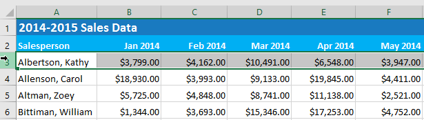
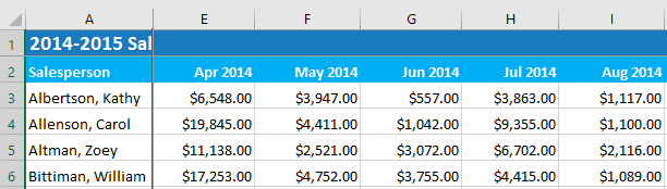
1. Select the row(s) below the row(s) you want to fix. For example, if you want to fix rows 1 and 2, then row 3 will be selected.

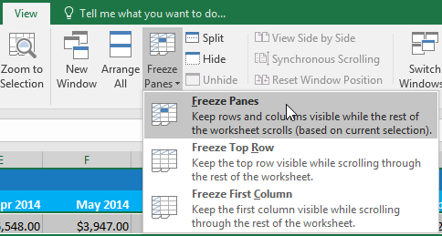
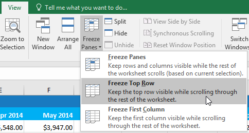
2. On the View tab , select the Freeze Panes command , and then select Freeze Panes from the drop-down menu.

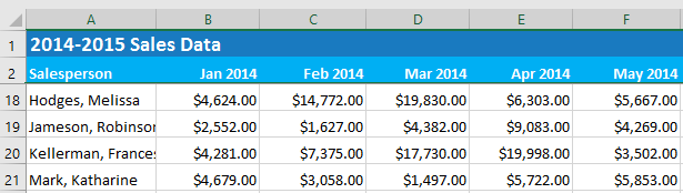
3. The rows will be fixed in place, as indicated by the gray line. You can scroll down the spreadsheet while continuing to view these fixed rows at the top. The example has scrolled down to row 18.

 

How to fix the columns

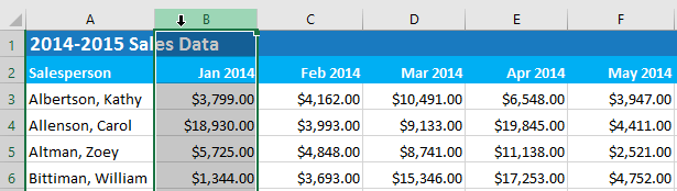
1. Select the column to the right of the column(s) you want to fix. For example, if you want to fix column A , then column B will be selected.

2. On the View tab , select the Freeze Panes command , and then select Freeze Panes from the drop-down menu.

3. The column will be fixed in place, as indicated by the gray line. You can scroll through the worksheet while continuing to see the fixed column on the left. For example, we have scrolled past column E.

If you only need to freeze the top row (row 1) or the first column (column A) in the spreadsheet, select Freeze Top Row or Freeze First Column from the drop-down menu.

 

How to unfix rows/columns

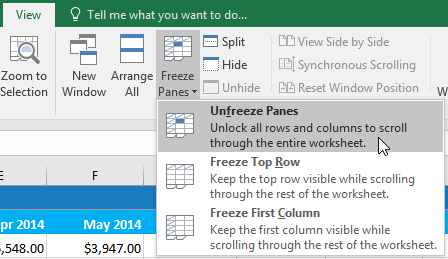
If you want to choose a different view option, you may first need to reset the spreadsheet by unfreezing rows/columns. To unfreeze rows or columns, click the Freeze Panes command , then select Unfreeze Panes from the drop-down menu.

Other view options

If your workbook contains a lot of content, it can sometimes be difficult to compare different sections. Excel includes additional options to make your workbook easier to view and compare. For example, you can choose to open a new window for your workbook or divide the worksheet into separate panes.

How to open a new window for the current workbook

Excel allows you to open multiple windows for a single workbook at the same time. This example will use this feature to compare two different worksheets from the same workbook.

1. Click the View tab on the Ribbon , then select the New Window command.

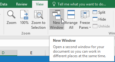
2. A new window for the workbook will appear.

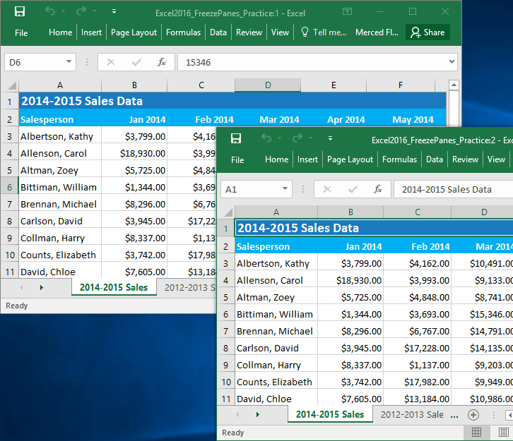
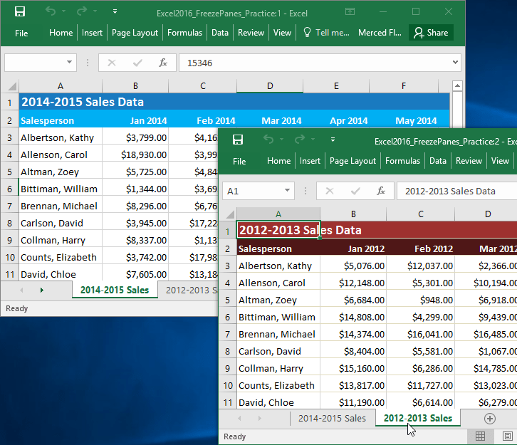
3. Now you can compare different worksheets from the same workbook across windows. For example, we would select the 2013 Sales Detailed View worksheet to compare sales figures for 2012 and 2013.

 

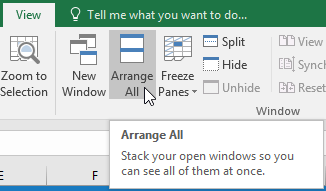
If you have multiple windows open at the same time, you can use the Arrange All command to quickly rearrange them.

How to split a worksheet

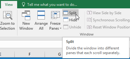
Sometimes, you might want to compare different sections of the same workbook without creating a new window. The Split command allows you to divide the worksheet into multiple separate scroll panes.

1. Select the cell where you want to split the spreadsheet. For example, we would select cell D6.

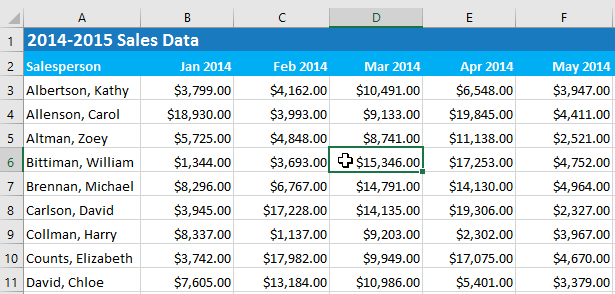
2. Click the View tab on the Ribbon , then select the Split command.

3. The workbook will be divided into different sections. You can scroll through each section individually using the scroll bars, allowing you to compare different parts of the workbook.

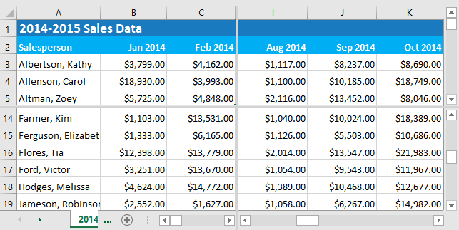
4. After separating, you can click and drag the vertical and horizontal dividers to resize each section.

5. To cancel the split, click the Split command again.