Excel 2019 (Part 20): Grouping and Subsummary

Spreadsheets with a lot of content can sometimes feel overwhelming and even become difficult to read. Fortunately, Excel can organize data into groups, allowing you to easily show and hide different parts of the spreadsheet. You can also summarize different groups using the Subtotal command and create outlines for your spreadsheet.

 

How to group rows or columns

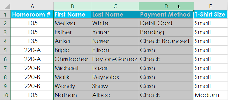
1. Select the rows or columns you want to group. This example will select columns B, C, and D.

 

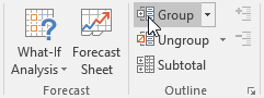
2. Select the Data tab on the Ribbon, then click the Group command.

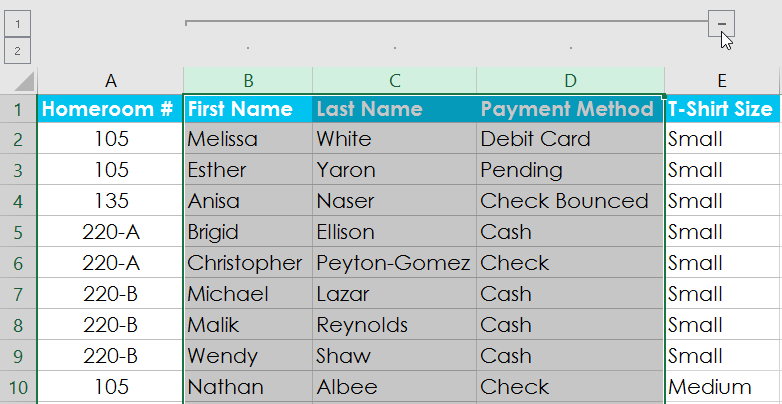
3. The selected rows or columns will be grouped together. In the example, columns B, C, and D are grouped together.

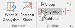
To ungroup data, select the grouped rows or columns, and then click the Ungroup command.

 

How to hide and show groups

1. To hide a group, click the minus sign, also known as the Hide Detail button.

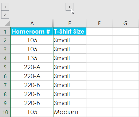
2. The group will be hidden. To show a hidden group, click the plus sign, also known as the Show Detail button.

 

Create subtotal

The Subtotal command allows you to automatically create groups and use common functions like SUM , COUNT , and AVERAGE to help summarize data. For example, the Subtotal command can help calculate the cost of office supplies by type from a large inventory order. It will create a hierarchy of groups, called an outline, to help organize the worksheet.

The data must be correctly sorted before using the Subtotal command, so you may want to review the article on Sorting Data for more information.

How to create a subtotal

For example, we'll use the Subtotal command with a t-shirt order form to determine the number of t-shirts ordered for each size ( Small, Medium, Large , and X-Large ). This will create an outline for the spreadsheet with each t-shirt size as a group and then count the total number of t-shirts in each group.

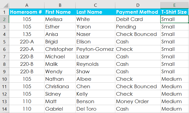
1. First, sort the spreadsheet by the data you want to subsum. This example will create a subsum for each t-shirt size, so the spreadsheet is sorted by t-shirt size from smallest to largest.

 

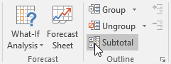
2. Select the Data tab , then click the Subtotal command.

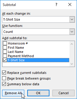
3. The Subtotal dialog box will appear. Click the drop-down arrow for the " At each change in:" field to select the column you want to subtotal. For example, we would select T-Shirt Size.

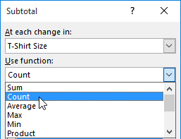
4. Click the drop-down arrow for the Use function: field to select the function you want to use. For example, we would select COUNT to count the number of shirts ordered by size.

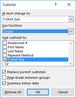
5. In the " Add subtotal to: " field , select the column where you want the subtotal to appear. For example, we would select "T-Shirt Size". When you are satisfied with your selections, click OK.

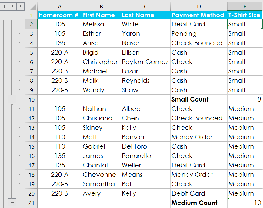
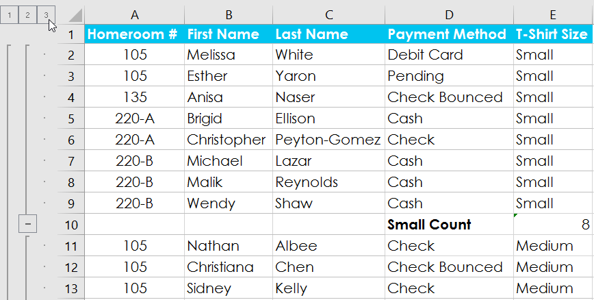
6. The spreadsheet will be divided into groups, and subtotals will be listed below each group. In the example, the data is currently grouped by t-shirt size, and the number of t-shirts ordered in that size appears below each group.

 

How to view groups by level

When you create subtotals, the worksheet is divided into different levels. You can switch between these levels to quickly control the amount of information displayed in the worksheet by clicking the Level buttons on the left side of the worksheet. The example will switch between all 3 levels in the outline. Although this example only contains 3 levels, Excel can actually contain up to 8 levels.

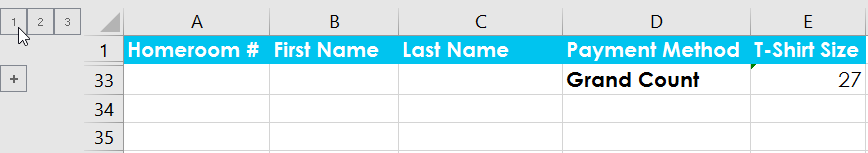
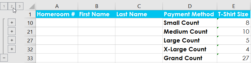
1. Click on the lowest level to display the least amount of detail. For example, level 1 would only contain the Grand Count or the total number of t-shirts ordered.

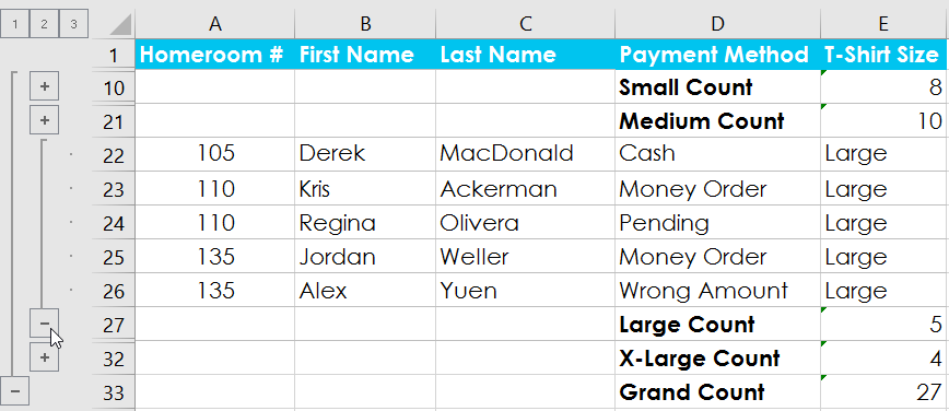
2. Click on the next level to expand the details. For example, level 2 would be selected, containing each subtotal row but hiding all other data from the worksheet.

3. Click on the top level to view and expand all the spreadsheet data. For example, we would select level 3.

You can also use the Show Detail and Hide Detail buttons to show and hide groups within the outline.

How to delete subtotals

Sometimes, you may not want to keep subtotals in your spreadsheet, especially if you want to reorganize the data in other ways. If you no longer want to use subtotals, you will need to delete them from your spreadsheet.

1. Select the Data tab , then click the Subtotal command.

 

2. The Subtotal dialog box will appear. Click Remove All.

3. All worksheet data will be ungrouped and subtotals will be deleted.

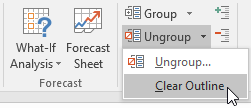
To delete all groups without deleting subgroups, click the Ungroup command drop-down arrow , and then select Clear Outline.