How to Filter Data in Excel 2019

Excel filters temporarily hide rows that do not meet selected criteria. They do not delete or move the records, so you can focus, copy, chart, or print a subset and then restore the full list.

The screenshots show Excel 2019. Recent desktop versions and Excel for the web use the same basic filter arrows, although menu details may vary.

Prepare data for reliable filtering

• Use one header row with a unique, nonblank name for each column.
• Keep the list rectangular, with no blank row or column splitting it.
• Store one data type per column. Do not mix real dates with text dates or numbers with numeric text.
• Avoid merged cells in the filter range.
• Convert a frequently expanding range to an Excel Table with Ctrl+T; table headers include filter controls automatically.

Filter by selected values

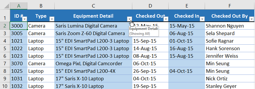
The example list has headers such as ID#, Type, Equipment Detail, and Checked Out.

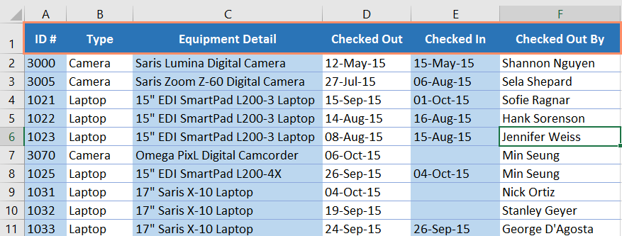
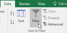
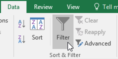
1. Select a cell inside the list, then choose Data > Filter. The shortcut Ctrl+Shift+L toggles filter controls for a normal range.

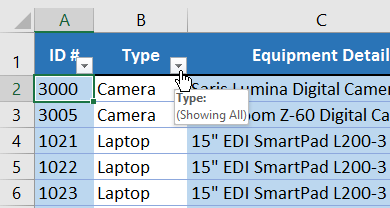
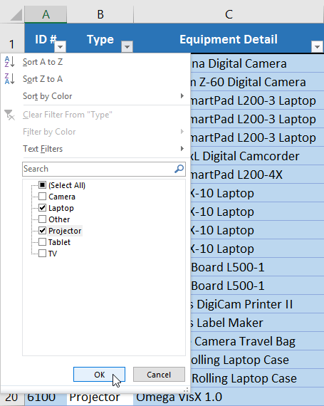
2. Open the arrow in the column to filter. Here, the Type column will be used.

3. Clear Select All.

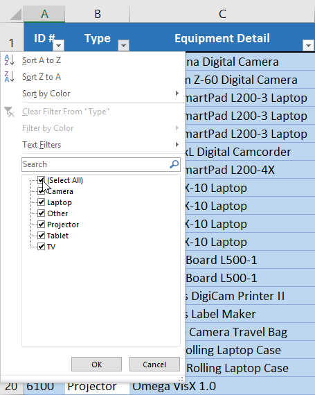
4. Select Laptop and Projector, then choose OK.

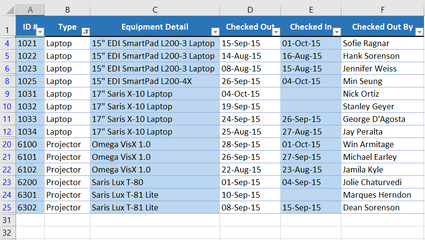
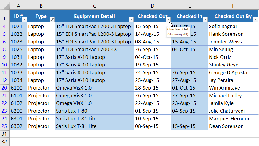
Excel displays only rows whose Type is Laptop or Projector. Row numbers may skip because the other rows are hidden by the filter.

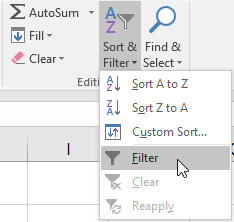
You can also enable and manage filters from Home > Sort & Filter.

Apply filters to more than one column

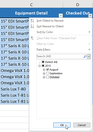
Filters in different columns are additive: a row must pass the Type filter and the Date filter. Open the Checked Out date column after filtering the device types.

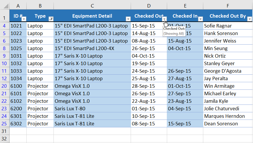
Select August and confirm.

The remaining rows are laptops or projectors whose date also falls in August.

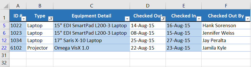
Within one checklist, selecting several values means OR. Across separate filtered columns, the relationship is AND. This distinction explains many unexpectedly empty filter results.

Clear one filter, all criteria, or the filter controls

Clear one column

Open the filter icon in the relevant header.

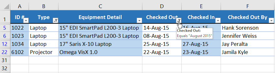
Select Clear Filter From “Checked Out”.

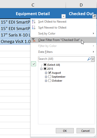
Rows excluded only by that date criterion reappear, while filters in other columns remain active.

Clear every active criterion

Use Data > Clear to show all rows while leaving the header arrows ready for another filter. This is usually preferable to turning filtering off.

Remove the filter arrows

Select Data > Filter again when you want to remove AutoFilter from the range entirely. This also redisplays the full list.

Filter with the search box

Open the filter arrow for the text column.

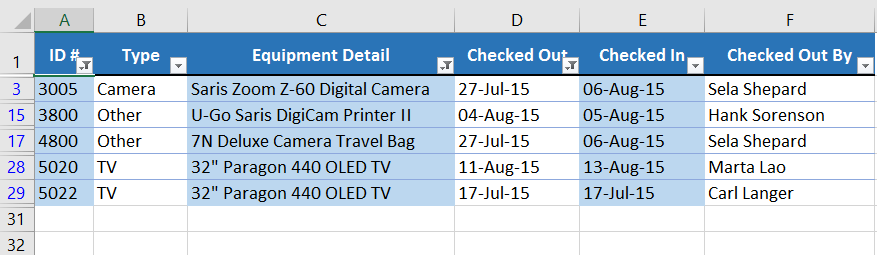
Type a term such as saris in the filter search box, review the matching values, and select OK.

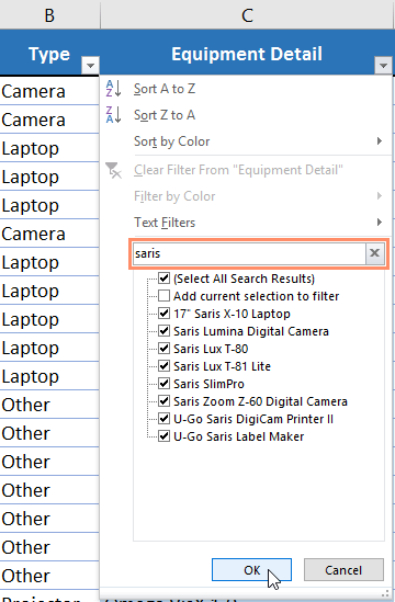
The sheet displays records whose selected column value matched the search.

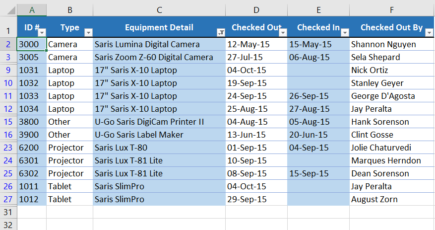
The filter-menu search works against unique values in that column and is not a replacement for the workbook Find command. With other column filters active, the available checklist may be limited to values still visible in the current subset. Excel’s filter window also does not list unlimited unique values, so use criteria filters when a value is absent from a very large list.

Use text criteria

Open the arrow for a text column.

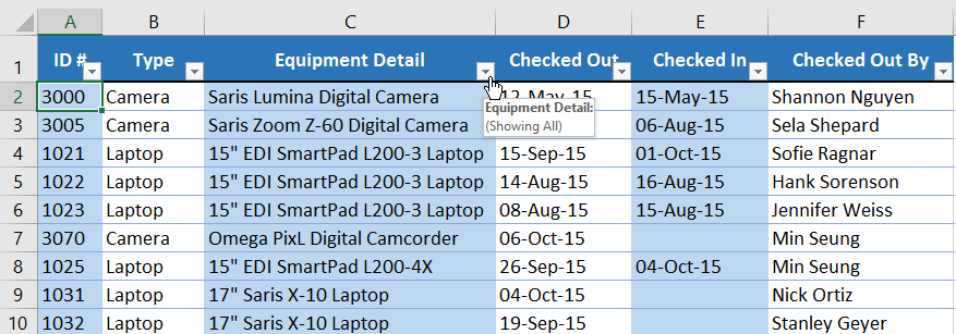
Choose Text Filters and an operator such as Equals, Does Not Equal, Begins With, Ends With, Contains, or Does Not Contain.

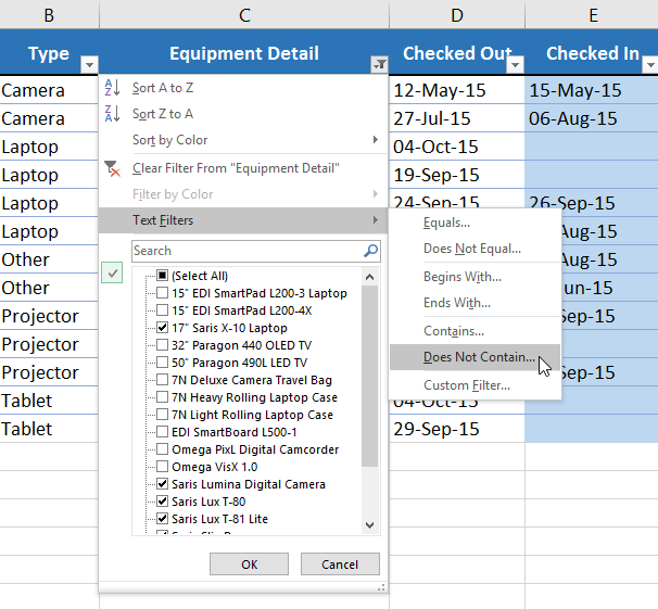
To exclude descriptions containing laptop, choose Does Not Contain, enter the word, and confirm.

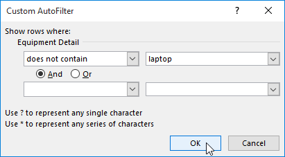
Excel displays rows whose selected text field does not contain that sequence.

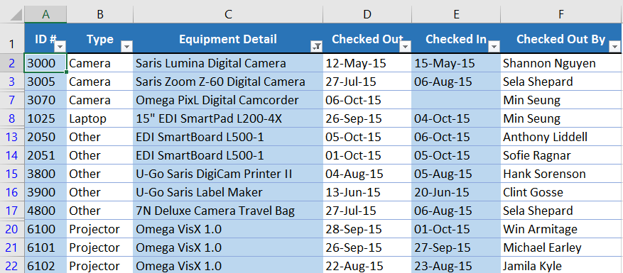
Custom AutoFilter can combine two criteria in the same column with And or Or. For example, Begins With “Pro” OR Begins With “Lap” includes either prefix. Blank cells require deliberate handling; a blank may appear as (Blanks) in the value list.

Use number criteria

Open the arrow in a genuinely numeric column.

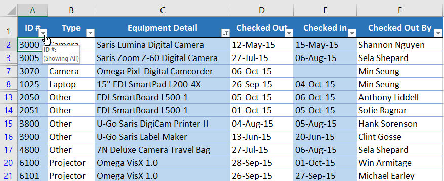
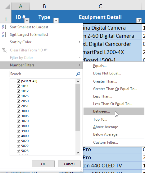
Choose Number Filters > Between or another comparison.

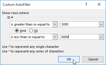
For an inclusive range of 3000 through 6000, use is greater than or equal to 3000 AND is less than or equal to 6000.

Only rows within the specified numeric range remain.

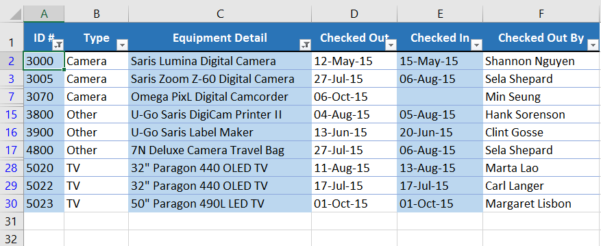
Identifiers are not always quantities. If an ID can contain leading zeros or letters, store it as text and use text filters instead of numeric comparisons. Filtering numeric IDs between two values is appropriate only when the numeric order has meaning.

Use date criteria

Open the arrow in a column containing real Excel dates.

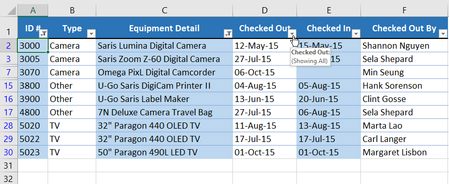
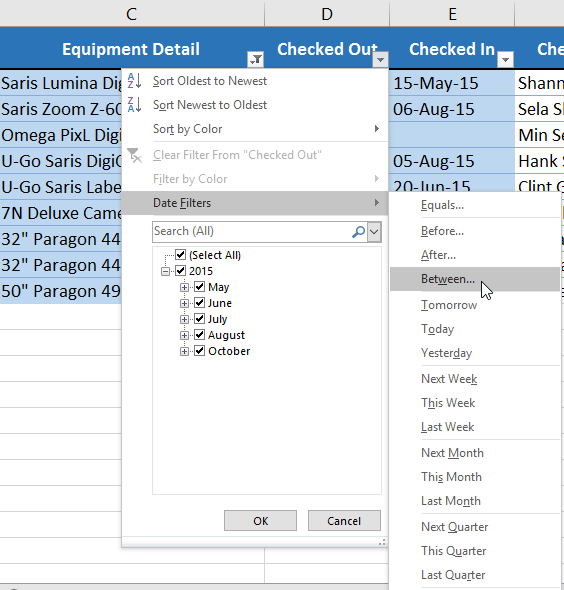
Choose Date Filters > Between.

Enter the start and end dates. In the example, both July 15, 2015 and August 15, 2015 are included.

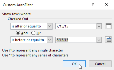
The filtered view contains records within that date range.

If Excel offers Text Filters instead of Date Filters, the column likely contains text or mixed types. Converting only the cell display format to Date does not convert date text into date values; clean the source values first. For date-time values with times, an end criterion of “less than the day after the final date” can be safer than “less than or equal to the final date,” which may include only midnight on that date.

Reapply after data changes

Changing a filtered cell, adding records, or recalculating formulas does not always refresh the visible subset immediately. Choose Data > Reapply after the source changes. If new rows are outside a normal filtered range, extend the range or use an Excel Table.

Work safely with filtered rows

• Check the status bar or visible row numbers before copying or deleting; hidden rows still exist.
• When pasting into a filtered list, verify whether Excel will affect hidden cells as well as visible cells.
• Use SUBTOTAL or another filter-aware summary when you need a total of visible rows. A plain SUM can include filtered-out values.
• Clear filters before using Find if you need to search the entire list; Find may search only displayed data in a filtered view.
• Do not infer that hidden rows are invalid records—they merely failed the current criteria.

Troubleshoot missing results

• Some rows were never included: a blank row split the original range, or new rows were added outside it.
• Wrong filter menu: the column contains mixed data types.
• Dates group incorrectly: some dates are text or include unexpected time values.
• Expected values are absent: another column filter has already narrowed the available subset.
• No rows remain: criteria in separate columns must all be true for a row.
• Filter buttons are unavailable: the sheet may be protected or the selection may be inside an unsupported layout.

For ordering rather than hiding rows, see how to sort Excel columns. For summary reports that users can filter interactively, build an Excel PivotTable. To mark exceptions while keeping every row visible, use conditional formatting in Excel.

Microsoft’s current references explain how to filter a range or table and how to clear or remove filters.