Table of Contents
Quick answer
The CRITBINOM function is a compatible function in Excel used to calculate the cumulative binomial distribution, commonly used in older versions such as Excel 2007. Below is the syntax and examples to help you understand how to use this function effectively in your work.
The CRITBINOM function returns the smallest value such that the cumulative binomial distribution is greater than or equal to a predefined criterion value.
Instructions on how to use the CRITBINOM function in Excel
Syntax : CRITBINOM(trials,probability_s,alpha)
In there:
- trials : Required – This is the number of Bernoulli trials.
- probability_s : Required – This is the probability of success for each trial.
- alpha : Required – This is the criterion value.
Note:
- If any parameter is not a number, the function will return a #VALUE! error. - If the trials
value is not an integer, it will be rounded down to an integer. - If trials is less than 0, the function will return a #NUM! error . - If the probability_s value is less than 0 or greater than 1, the function will return a #NUM! error . - If alpha is less than 0 or greater than 1, the function will return a #NUM! error.
Consider the example
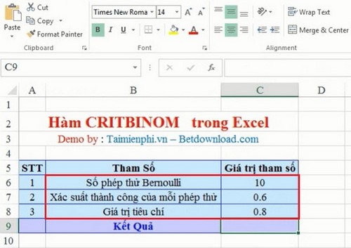
You enter your actual values corresponding to the function parameters into the Excel cells. In this example, the number of Bernoulli trials is 10, the probability of success for each trial is 0.6, and the criterion value is 0.8.
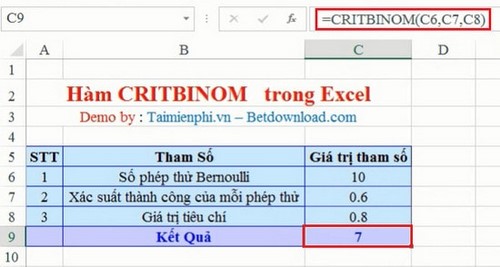
Enter the formula in cell C9. And the result of the function is 7.
So now you know how to use the CRITBINOM function in Excel. When entering parameters, make sure the arguments are numeric. If the number of Bernoulli trials is not an integer, Excel will automatically truncate the number for calculation.
The CRITBINOM function is combined with the COUNTIF and HLOOKUP functions.
When you have a list of names and need to count the number of occurrences in the table according to a specific requirement, the COUNTIF function will help you do that. The COUNTIF function allows you to count the number of occurrences based on a given condition.
If you have a transcript and academic ranking criteria for students, you will need to use the HLOOKUP function. The HLOOKUP function will retrieve the results that meet the criteria and then assign the corresponding academic ranking to the eligible students.
Related Articles
 The Index Function in Excel: Formulas and Usage9 minutes read
 How to use the VALUE function in Excel - A function to4 minutes read
 Basic Excel Functions That Anyone Must Know20 minutes read
 How to Use Hlookup Function on Excel: Excel Hlookup Function4 minutes read
 How to Use the SUM Function to Calculate Totals in Excel8 minutes read
 DATE Function: Converts Numbers to a Valid Date Format5 minutes read
Reader Comments 0
Sign in with email or Google to join the discussion.