How to use the VSTACK and HSTACK functions in Excel

Combining multiple data files, merging columns or rows, and creating a unified view of information is possible with two powerful functions in Excel: VSTACK and HSTACK, which simplify this process without having to write complex formulas.

What are the VSTACK and HSTACK functions? How to use them in Excel?

 

I. What are the VSTACK and HSTACK functions?

- VSTACK and HSTACK are two new functions in Excel that allow users to append data and stack it horizontally or vertically. Both functions use a dynamic array environment to add data and stack it as lists, specific header arrays, etc.

- Because both are new Excel functions, only Microsoft 365 users can use them to improve work efficiency.

 

II. Syntax and Usage of the VSTACK Function in Excel

1. Syntax of the VSTACK function in Excel

- Syntax of the VSTACK function: =VSTACK(array_1, [array_2], .)

- In this case, "array_1" is a reference to the required data range; the following arrays are optional.

2. How to use the VSTACK function in Excel

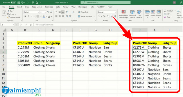
- Suppose you have two tables as shown below and want to merge the data from both horizontally using the VSTACK function:

+ In the formula bar, enter =VSTACK(

+ Then, write the array for the first table and add a comma. Taimienphi's first table is B4:D8

After the comma, fill in the next array for the second table: F4:H8 , close the parenthesis and press Enter on the keyboard.

The final syntax for VSTACK in Excel is =VSTACK(B4:D8,F4:H8) , with the result as shown below.

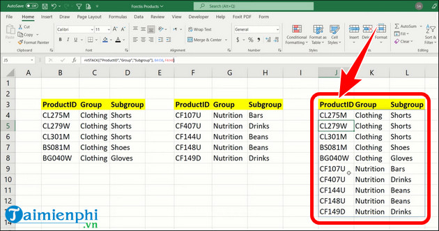
- In addition to the above usage, you can also merge two data ranges and static arrays directly within the VSTACK function in Excel. Specifically:

=VSTACK({"ProductID", "Group", "SubGroup"}, B4:D8, F4:H8)

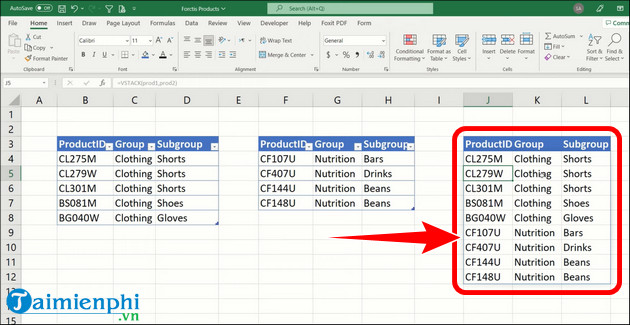
- Additionally, readers can merge data tables together, and when new data is added, the VSTACK function will automatically update its results.

+ In the formula bar, enter =VSTACK(

+ Write the first table " prod1 " and add a comma to separate the tables " prod2 ", close with parentheses and press the Enter key on the keyboard.

Result: =VSTACK(prod1,prod2)

 

III. Syntax and Usage of the HSTACK Function in Excel

1. HSTACK function syntax in Excel

- Standard syntax for the HSTACK function: =HSTACK(array_1, [array_2], .)

- Similar to the VSTACK function, array 1 is a required parameter and is a reference to the data range, while array 2 is optional.

- While the VSTACK function joins data and stacks it horizontally, the HSTACK function does the opposite and stacks it vertically.

2. How to use the HSTACK function in Excel

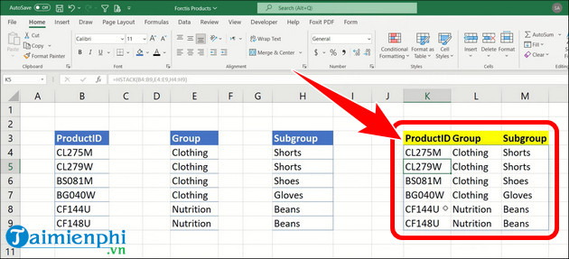
For example, you have three tables: ProductID, Group, and Subgroup, as shown below. To make it more concise, you can merge the data from all three tables using the HSTACK function.

+ In the formula bar, enter =HSTACK(

+ Fill in the data from Table 1 to Table 3 and add commas to separate the arrays.

The final syntax for this example would be =HSTACK(B4:B9,E4:E9,H4:H9) . This will be followed by the result displayed on the screen.

Through the examples above, readers should now understand how to use the VSTACK and HSTACK functions in Excel. This will allow you to apply the formulas to your work most effectively.

In Excel, the VLOOKUP function is also commonly used to search for values ​​by column and return results vertically. This is a very popular and convenient function for users who frequently use Microsoft Excel.