How to use the Vlookup function in combination with the Left function.

Combining functions in Excel makes calculations easier and more accurate. The VLOOKUP function looks up information based on a condition, while the LEFT function extracts characters from the left side of a string.

 

INSTRUCTIONS ON HOW TO USE THE VLOOKUP FUNCTION IN COMBINATION WITH THE LEFT FUNCTION

Syntax and usage of the VLOOKUP and LEFT functions

The VLOOKUP function: Used to look up and return results vertically.

- Syntax: =VLOOKUP(lookup_value, table_array, col_index_num, [range_lookup])

+ lookup_value: The value to look up

+ table_array: The data range to look up

+ col_index_num: The column order from which to retrieve data

+ range_lookup: Search range, TRUE (relative lookup) or FALSE (absolute lookup)

Notes on using F4:

- F4 (once): Fix both column and row ($A$8)

- F4 (twice): Fix row, not column (A$8)

- F4 (3 times): Fix column, not row ($A8)

The LEFT function is used to extract the characters from the left side of a string.

- Syntax: =LEFT(text, n)

+ text: The string of characters to be extracted

+ n: Number of characters to cut

We will use examples to better understand how to use and combine these two functions.

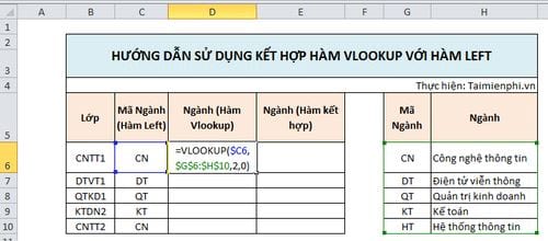
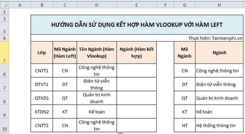
Let's assume we have a data table like the one below:

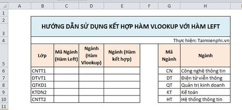
We will use the LEFT function to retrieve the Department Code from the Class column.

Step 1 : Fill in cell C6 with the formula: =LEFT(B6,2). The meaning of this formula is to remove 2 characters from cell B6.

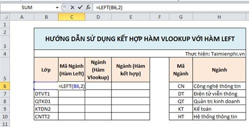
Step 2: Then press Enter . The result will be the two characters CN that have been extracted from the string CNTT1 .

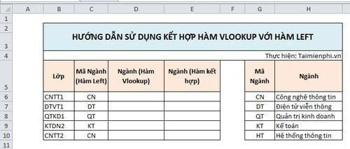
Step 3 : Drag from cell C6 downwards so that the cells below automatically fill in the formula and display the corresponding result.

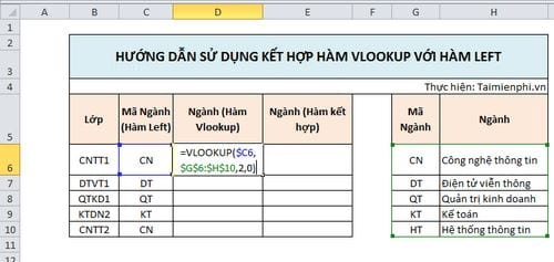
Step 4: Fill in cell D6 with the formula: =VLOOKUP($C6,$G$6:$H$10,2,0). $C6 is the value to search for, $G$6:$H$10 is the data range to look up, 2 is the column number to retrieve the value from within the data range, and 0 is the absolute search range.

Step 5: Then press Enter . The result will show the Department Name corresponding to the Department Code . Scroll down again so that the cells below automatically fill in the formulas and give the corresponding results.

Step 6: Fill in cell E6 with the formula: =VLOOKUP(LEFT(B6,2),$G$6:$H$10,2,0). We replace the value used for searching from $C6 with LEFT(B6,2) .

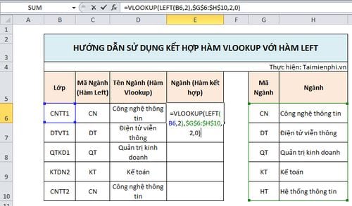
Step 7: Then press Enter and do the same as step 5.

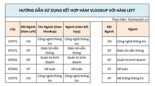
Above is how to combine the VLOOKUP function with the LEFT function. Hopefully, this article helps you use these functions effectively in your work. If you encounter any difficulties, don't hesitate to leave a question below the article, and the TipsMake team will assist you.

Besides being combined with the LEFT function, the VLOOKUP function can also be combined with the IF function to solve other problems. You can refer to how  to combine the VLOOKUP and IF functions  to find data based on conditions here.