How to Use the SUMIF Function in Excel

SUMIF adds values that meet one condition. The condition can test numbers, text, dates, blanks, or patterns. Use SUMIFS instead when every row must satisfy two or more conditions.

SUMIF syntax

=SUMIF(range,criteria,[sum_range])

• range: cells Excel tests.
• criteria: the required condition.
• sum_range: cells to add. If omitted, Excel adds matching cells in range.

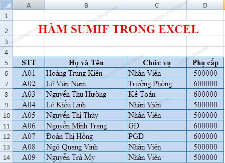
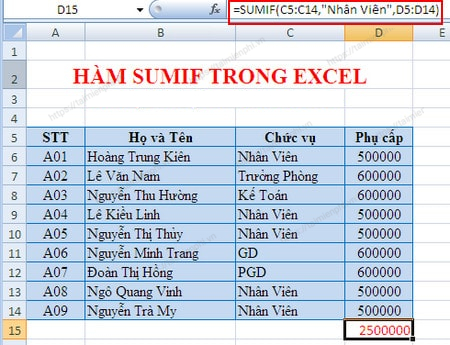
For example, to total allowances in D5:D14 where C5:C14 contains “Employee”:

=SUMIF(C5:C14,"Employee",D5:D14)

Numeric comparisons

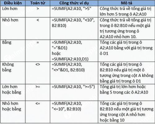
Put comparison operators inside quotation marks:

• =SUMIF(B2:B20,">=60",C2:C20)
• =SUMIF(B2:B20,"<100",C2:C20)
• =SUMIF(B2:B20,"<>0",C2:C20)

Text criteria and cell references

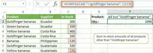
SUMIF is not case-sensitive. This formula excludes one exact product name:

=SUMIF(A2:A8,"<>Goldfinger bananas",C2:C8)

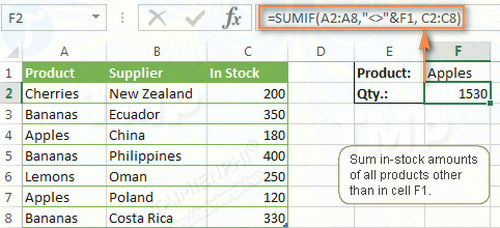
To take the excluded product from F1, concatenate the operator and reference:

=SUMIF(A2:A8,"<>"&F1,C2:C8)

Partial matches with wildcards

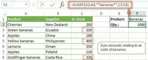
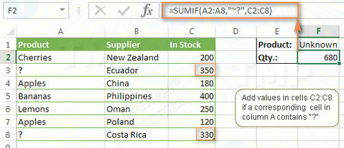
• * matches any sequence of characters.
• ? matches one character.
• ~ makes the following * or ? literal.

=SUMIF(A2:A8,"*banana*",C2:C8) sums rows whose text contains “banana.” To take the word from F1, use =SUMIF(A2:A8,"*"&F1&"*",C2:C8).

To match a literal question mark, use =SUMIF(A2:A8,"~?",C2:C8).

Sum rows with blank or nonblank criteria

To add C2:C10 where the corresponding A cell is blank:

=SUMIF(A2:A10,"",C2:C10)

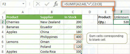
For nonblank corresponding cells, use =SUMIF(A2:A10,"<>",C2:C10). Be cautious with formulas that return an empty string: spreadsheet functions may treat these differently from truly empty cells.

Use dates in SUMIF

Dates should be real Excel dates, not text. A cell reference is safer than typing a locale-dependent date:

=SUMIF(B2:B20,">="&F1,C2:C20)

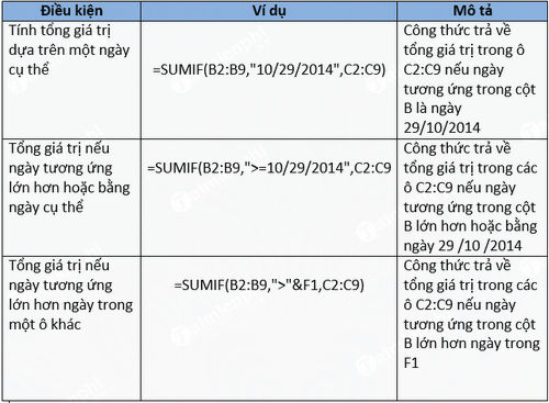
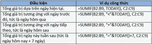
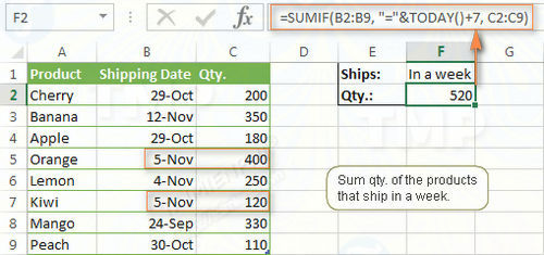
For today's date, concatenate TODAY(): =SUMIF(B2:B20,TODAY(),C2:C20). Other comparisons use forms such as "<"&TODAY().

Sum between two dates

SUMIFS expresses a date interval more clearly. If F1 is the start date and G1 is the end date:

=SUMIFS(C2:C20,B2:B20,">="&F1,B2:B20,"<="&G1)

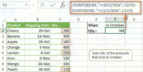
If B contains date-and-time values, an inclusive “less than or equal to end date” condition may miss times later that day. One robust pattern is to use "<"&G1+1.

Sum across several value columns

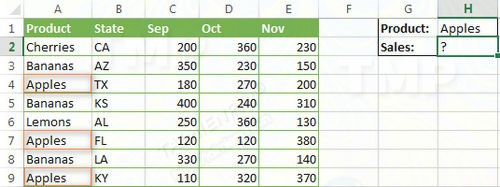
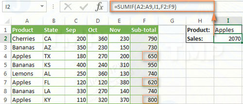
SUMIF expects sum_range to align with range. When each product has monthly values across C:E, first total each row in helper column F with =SUM(C2:E2), then use:

=SUMIF(A2:A9,H1,F2:F9)

Why SUMIF returns the wrong result

• Make range and sum_range the same size and shape.
• Check numbers or dates stored as text.
• Remove unintended spaces from text criteria.
• Join operators to cell references with &.
• Use SUMIFS for multiple conditions instead of subtracting several hard-to-audit formulas.
• Confirm the workbook's regional argument separator: some installations use semicolons.

For a focused diagnostic checklist, see SUMIF errors and fixes. For conditional counting rather than summing, use the COUNTIF function.