How to make a thermometer template in Excel

Using a thermometer chart in Excel is a good choice for keeping track of financial goals. Here is a detailed step-by-step guide on how to make a heat chart in Excel .

How to make a thermometer template in Excel Picture 1

Whether you're planning a vacation, running a marathon, or saving money to build the home of your dreams, you'll want to keep track of your progress.

A good way to do this is to use a thermometer chart in Excel. It is a simple, effective way to track a financial goal and share it with your team, partners or friends.

Spreadsheet Setup

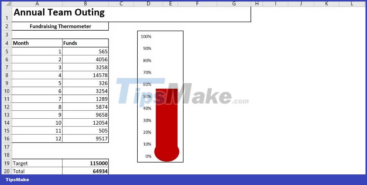
Before making the thermometer, we need to set the goal. In this case, look at the plan to track funds for a group trip.

1. Open a new worksheet in Excel.

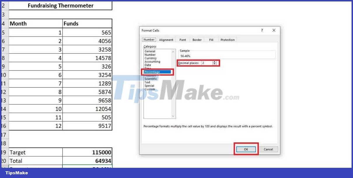
2. Create an Excel table with 2 columns: one for Month and one for Amount Deposited .

3. Below the table, pay attention to the cells: Target , Total and Percentage . Here, we will create formulas for thermometers.

How to make a thermometer template in Excel Picture 2

4. Next to Target , enter the target amount in column B. The target here is 115,000 USD.

5. Next to Total , write the formula:

=Sum(B5:B16)

This formula shows the amount collected in column B.

6. Finally, we can calculate the percentage by:

=B20/B19

Enter it in column B21.

7. Change the format to percentage by right-clicking on the cell and selecting Format Cells . Change the directory to Percentage , select the number of decimal places you want to display and press OK .

How to make a thermometer template in Excel Picture 3

Create a heat chart in Excel

1. Click the Insert tab .

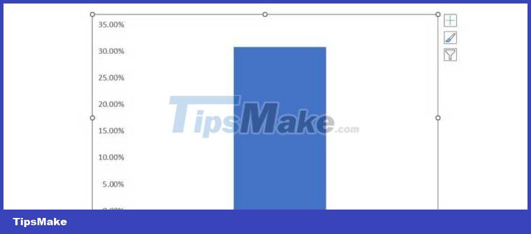
2. In the charts section , click insert column or bar chart and select 2-D Clustered Column .

How to make a thermometer template in Excel Picture 4

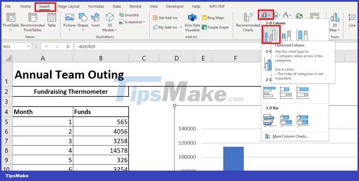
This action will create a chart next to your table.

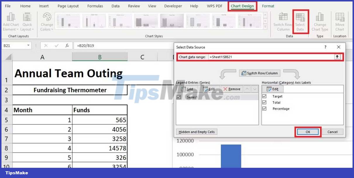
3. Next, add the table to the chart using Select Data . Select the cell that contains the percentage of the total. Click OK to populate the chart.

How to make a thermometer template in Excel Picture 5

4. You can now split the chart. Right click on the chart name and delete it. Do the same for column headers and horizontal lines.

How to make a thermometer template in Excel Picture 6

Note: If you don't want to delete them, you can hide the chart axes in Excel.

5. Double-click the y-axis to open the dialog box. From here, you can change the chart's minimum and maximum limits to 0.0 and 1.0 respectively. Before closing the menu, select Numbers and change the decimal place to 0.

How to make a thermometer template in Excel Picture 7

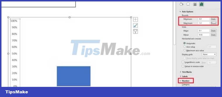
6. Right-click the column and select Format Data Series . Adjust the Gap Width to 0 .

This action ensures your column fills the chart area, rather than trying to hide in the corner. You can now shrink the chart to a thermometer-like size.

7. Finally, go back to the Insert tab , select Shapes and find a nice oval shape. Draw an oval and add it to the bottom of the heat chart, then resize the chart area. It should fit snugly around the round end of the thermometer, such as:

How to make a thermometer template in Excel Picture 8

Note: You can change the thermometer to red by right clicking on the colored part and changing the fill color.

Add details to a heat chart in Excel

If you're tracking large amounts of money in a long-term plan, it can be helpful to review the date of the biggest increase, especially in philanthropic activities. From there, you can analyze your team's performance.

First, change the Excel table. You need more details, including the date and name of the donor. You need to separate the date and received amount columns. This way you can monitor each variable.

Next, you need to set up Dynamic Named Range. Named ranges are useful in providing control over a group of cells without having to update the formula. You can automatically request formulas for any data added to the table.

Dynamic Named Range settings

To make things easier later, make your board a full-fledged board. Do this by selecting the entire table area. Select Format as Table , and then select the style you want. Check the box next to My Table Has Headers and click OK .

You now have a searchable table with headers. Next, we can link the table to the totals (cell B20).

1. In the totals box, enter:

=SUM(Table1[Amount])

This formula requires the cell to calculate the Amount column . The percentage information remains the same, by dividing the total by the goal, and is still linked to the thermometer.

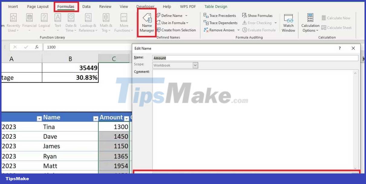
2. Select the contents of the Amount column (C26:C41) .

3. Select the Formulas tab and define the Name Manager . Click New .

4. In the Refers to box , you'll see =Table1[Amount] . You need to add the formula below so that each time you add a value to the Amount column , your total will automatically increase.

=OFFSET(Sheet1!$C$1,0,0,COUNTA(Sheet1!$C:$C),1)

The formula will look like this:

How to make a thermometer template in Excel Picture 9

Adding dates using SUMIFS

SUMIFS is a powerful formula that allows comparing information from two or more sources. Use the SUMIFS function to calculate the number of donations in 14 days. The result will look like this:

1. Enter the start date (cell G26).

2. In cell G27, type:

=G26+14

Excel will automatically insert the date for you and keep updating it based on cell G26.

3. G28 will contain the SUMIFS formula. In this box, type:

=SUMIFS($C$26:$C$95,$A$26:$A$95,">="&$G$26,$A$26:$A$95,"<="&$G$27)

4. Now, cell G28 will represent the value of the donations received between the dates you specified.

It's done!

Above is how to draw a thermometer chart in Excel . Hope the article is useful to you.

Samuel Daniel

Update 27 June 2023