MINVERSE function - The function returns the inverse matrix of a given matrix in Excel

Usually the process of calculating the inverse matrix of a given matrix is ​​very confusing and manual calculations take a lot of time. The following article shows how to use the MINVERSE function in Excel, which returns the inverse matrix of a given matrix.

Description: The function returns the inverse matrix of a given matrix.

Syntax: MINVERSE (array) .

Inside:

- array is an array with equal number of rows and columns.

Example: Find the inverse matrix of the following matrix:

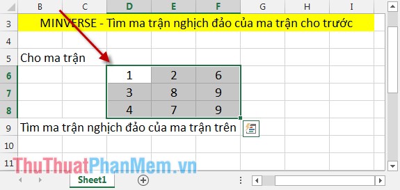
Step 1: In the cell to calculate the inverse matrix, enter the formula: MINVERSE (D6: D8) .

Step 2: After entering the formula, press Enter to get the results:

Step 3: Highlight the data area from D11: F13 (note the number of rows and highlighted columns depending on the original size of the matrix) -> Press F2 to get the results as shown:

Step 4: Press the key combination Ctrl + Shift + Enter to get the results:

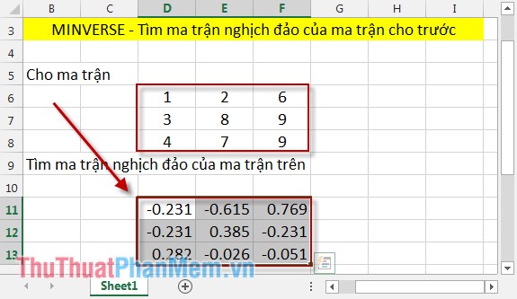
Thus, with a simple operation, you can immediately find the inverse matrix of a given matrix.

Good luck!