Table of Contents
This guide explains how to use FISHERINV Function in Excel, including its syntax, required arguments, practical examples, and common errors.

Description: The function returns the inverse value of the Fissher transformation . Use this function to analyze the correlation between two data arrays, if y = FISHER (x) -> FISHERINV (y) = x .
Syntax: FISHER (y)
Inside:
- y: The numerical value to perform the inverse of the Fissherinv transformation.
Attention:
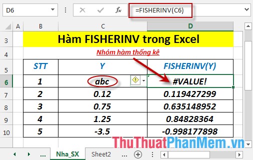
- If y is not a number -> the function returns the #VALUE! Error value.
- Fissherinv transform equation is:
[x = frac {{{e ^ {2y}} - 1}} {{{e ^ {2y}} + 1}}]
For example:
Calculate the inverse value of y after performing the fissherinv transformation using the data in the following data table:

- In the cell to calculate enter the formula : = FISHERINV (C6)
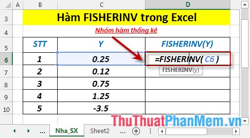
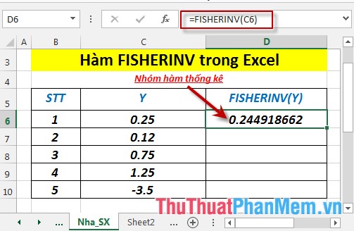
- Press Enter -> the inverse value of y after performing the fissherinv transformation is:
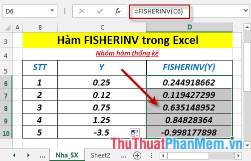
- Similarly copy to the remaining values are results:
- Where y is not a numeric form -> the function returns the #VALUE! Error value
Above are instructions and some specific examples when using FISHERINV function in Excel.
Good luck!
FAQ
What does the FISHERINV function do in Excel?
The FISHERINV function performs the calculation described in this guide. Use the correct arguments and compatible data types for reliable results.
How do I enter the FISHERINV function correctly?
Start with an equals sign, enter FISHERINV, add the required arguments inside parentheses, and confirm that cell references and separators are correct.
Why does the FISHERINV function return an error?
Common causes include missing arguments, invalid data types, incorrect cell references, unsupported values, or regional separator settings.





Reader Comments 0
Sign in with email or Google to join the discussion.