CUMPRINC function - The function calculates the cumulative capital amount payable in Excel

In the process of investing and calculating, if you do not have enough capital, you will definitely need to borrow to invest. Once you have borrowed the investment you want to calculate how much debt to pay off at the end of the term. The following article shows how to use the CUMPRINC Function to help you calculate by calculating the cumulative capital amount to pay.

Description: The function returns the cumulative capital amount of a loan from the beginning of the period to the end of the period, usually the function returns a negative value because the value of the function represents the amount of money lost due to borrowing.

Syntax: CUMPRINC (rate, nper, pv, start_period, end_period, type) .

Inside:

- rate : The interest rate of each period, is a required parameter.

- nper : Total number of periods with interest payment, a required parameter.

- pv : The value of the loan amount at the present time, is the required parameter.

- start_period : The first of the periods in which you want to calculate the cumulative capital amount, is the required parameter.

- end_period : The last of the periods in which you want to calculate the cumulative capital payables, is the required parameter.

- type : Method of interest payment, if type = 0 => interest paid at the end of the period, type = 1 => interest paid at the beginning of the period.

Attention:

- rate, nper must use a consistent unit, for example, loan is annualized => interest is calculated by year.

- If nper, end_period, start_period, type are decimal => the function takes the integer value of the above parameters.

- If the function pv returns the #NUM!

- If start_period <1, end_period end_period => the function returns the value #NUM !.

- Because the type has only 2 values, 0 and 1 if the parameter is outside these 2 values ​​=> the function returns the value #NUM !.

For example:

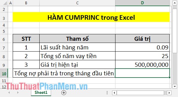
Calculate the total liabilities of the loan below in the first month and in the second year with the following table:

CUMPRINC function - The function calculates the cumulative capital amount payable in Excel Picture 1

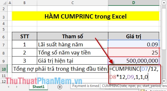
1. Calculate the total amount of liabilities payable in the first month

Since the interest rate is per year, it is necessary to divide the interest rate by 12 months, the total loan amount by the year, so the number of years times 12.

In the cell to calculate enter the formula: = CUMPRINC (D7 / 12, D8 * 12, D9,1,1,0) .

CUMPRINC function - The function calculates the cumulative capital amount payable in Excel Picture 2

Result:

CUMPRINC function - The function calculates the cumulative capital amount payable in Excel Picture 3

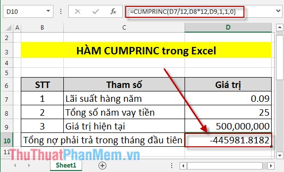
Because it's a debt, it has a negative value.

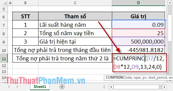
2. Calculating liabilities in the second year

In 2nd year starting from the expiry of the period 13 to 24. So why should count box enter the following formula: = CUMPRINC (D7 / 12, D8 * 12, D9,13,24,0) .

CUMPRINC function - The function calculates the cumulative capital amount payable in Excel Picture 4

Result:

CUMPRINC function - The function calculates the cumulative capital amount payable in Excel Picture 5

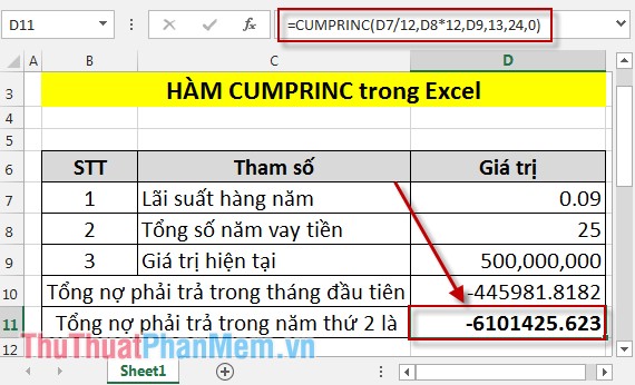
Because the debt calculation should be negative. So with CUMPRINC function you will identify the debt you have to pay when the loan helps you adjust your work arrangements.

Good luck!