Lock a Range of Data on Excel Spreadsheets

This article provides a clear overview of Lock a Range of Data on Excel Spreadsheets, with the main facts, useful context, and practical details organized for easy reading.

this guide shows how to lock the data area on Excel worksheet, you do as follows:

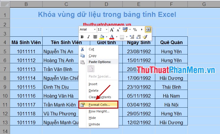
Step 1: Open the sheet containing the data area to lock, then select all the sheets by pressing Ctrl + A. Then right-click and select Format Cells .

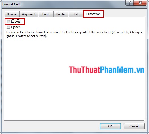
In the Format Cells dialog box, select the Protection tab and uncheck Locked and click OK .

Step 2: Select the data area to lock, then right-click and select Format Cells .

Reappears the Format Cells dialog box, select the Protection tab, select Locked and click OK .

Step 3: You can choose Review -> Protect Sheet (or Home -> Format -> Protect Sheet ).

The Protect Sheet dialog box appears, enter the password in the Password to unprotect sheet box -> OK .

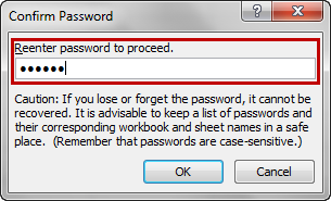
Confirm the password in Reenter password to proceed -> OK .

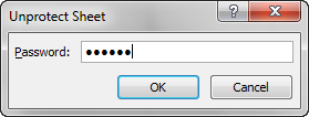
So your data area is locked, to unlock you go back to Review -> Unprotect Sheet (or Home -> Format -> Unprotect Sheet ) then enter the password into the Unprotect Sheet dialog box and click OK to open. Data area lock.

Thus, with very simple actions, you can quickly lock the necessary data area so that other people cannot edit the data in it. But you need to remember the password to unlock when you need to fix it. Good luck!