How to use the AVERAGE function in Excel

In Excel's basic functions, a group of functions functions as SUM functions and Average functions, etc. are used by many people. The Average function on Excel is used to calculate the arithmetic mean of a sequence of numbers in nature, supporting faster calculations in long numbers. Average function syntax as well as very simple, uncomplicated usage such as the conditional averaging function Averageif in Excel. The following article will show you how to use the Average function in Excel.

1. How to combine Sumif and Vlookup functions in Excel
2. 
   How to use Lookup function in Excel
3. How to use Vlookup function in Excel

1. How to use the Average Excel function

Average function syntax is = AVERAGE (number1, [number2], .) .

Inside:

1. number1: The first argument can be the number, cell reference or range containing the number you want to average, required.
2. number2: is the number, cell reference or range containing additional numbers that you want to calculate up to 255 numbers, optional.

Users should note when using:

1. AVERAGE has a maximum of 256 arguments, which can be numbers, names, ranges or cell references containing numbers.
2. The cell reference parameter or range contains a logical, text, or empty value, the function is automatically omitted, the value 0 alone will be calculated.
3. Logical values, denoting the text as numbers when entering directly into the list of arguments in the function will be counted.
4. If the argument is text or the value cannot be converted to a numeric form, an error will occur.

We will take the example with the data table below, averaging the scores for each student.

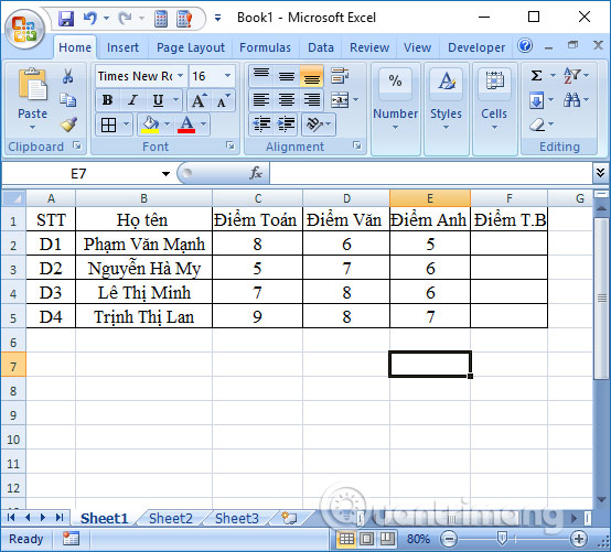
Step 1:

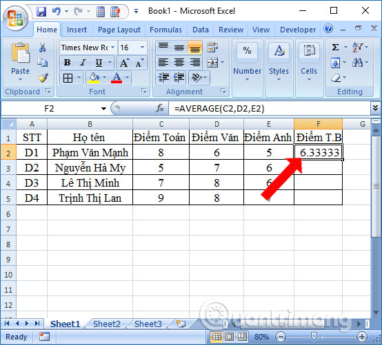
In the first average score box for the first student, the user enters the formula = AVERAGE (C2, D2, E2) and then press Enter.

Step 2:

The result will be displayed as shown below. In the case of decimal results as shown and want to round, the reader should refer to the article How to round numbers in Excel.

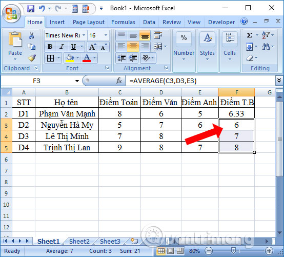
To calculate the average of the next cells, users simply point to the first result box and drag down the cells below.

2. Fix #VALUE error using Average function

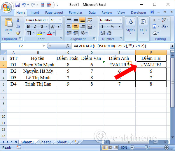
While using the Average function to calculate the average of data on Excel, users will encounter some common errors such as reporting the #VALUE! Error. This error occurs when the argument in the calculation that the Average function cannot interpret those values ​​is a numeric value.

With the image below, cell F2 is reporting a #VALUE! Error. because in the calculation, cell E2 contains the #VALUE value.

To fix the #VALUE! Error, you need to use two IF functions and the ISERROR function to ignore the reference area containing the error, to average the remaining normal values.

The function formula is = AVERAGE (IF (ISERROR (C2: E2), "", C2: E2)) .

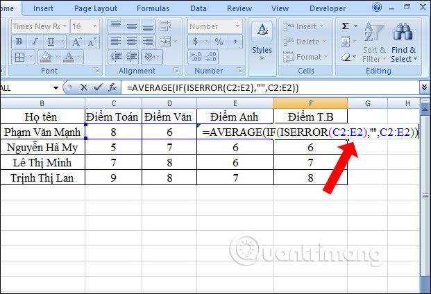
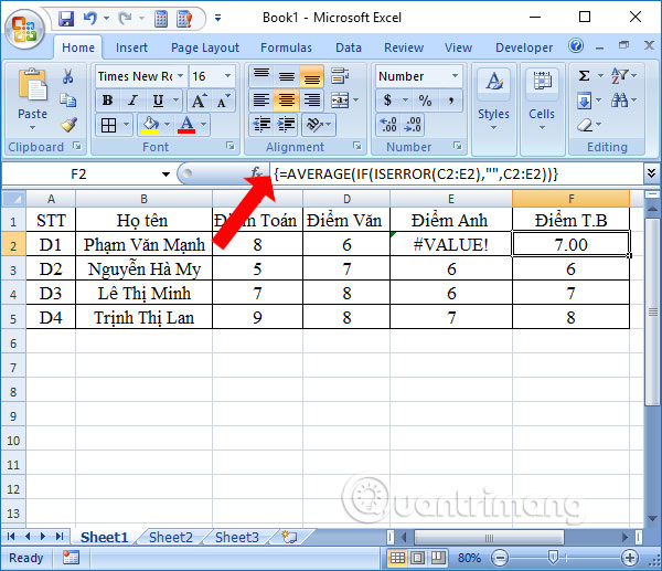
Since this is an array formula, users need to enter Ctrl + Shift + Enter to display the first and second brackets. If there are no parentheses the result will still report an error.

The result will be displayed as below. Cell E2 will not be included in the calculation.

Above is how to use the Average average function on Excel. The implementation is very simple, just need to localize the data you need to calculate. Also how to fix #VALUE! The above can be applied to # N / A, #NULL, # p / 0! errors, . of the Average function.

See more:

1. How to use ConcateNate function on Excel
2. How to use SUMPRODUCT function in Excel
3. How to use the DAVERAGE function in Excel

I wish you all success!