How to Multiply Numbers in Google Sheets

This updated guide examines How to Multiply Numbers in Google Sheets and organizes the essential facts, background, and practical takeaways in clear American English.

• 6 useful functions in Google Sheets you may not know
• How to link data between spreadsheets in Google Sheets
• How to use the AVERAGE function in Google Sheets

Multiply two integers together

There are two ways to multiply two numbers together. One is to use the integrated formula and the other is to use the multiplication operator to complete the calculation. Both ways work almost the same.

Use the MULTIPLY formula

Open a browser, access Google Sheets and open a spreadsheet.

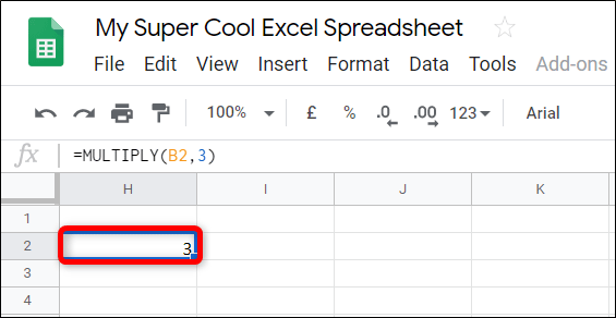
Click in the empty box and type=MULTIPLY(,), replace and with the integer you want to multiply.

You can also use data inside other cells. Instead of typing the numbers, type the number of the cell and Sheets will automatically fill the whole number with that cell in the correct position.

After setting the number or cell number, press Enter to display the result in that cell.

Use the operand

This method uses the multiplication operator (*) to find the product of numbers. The difference from the above method is that you can enter more than two numbers multiplied, while the previous formula is limited to two numbers.

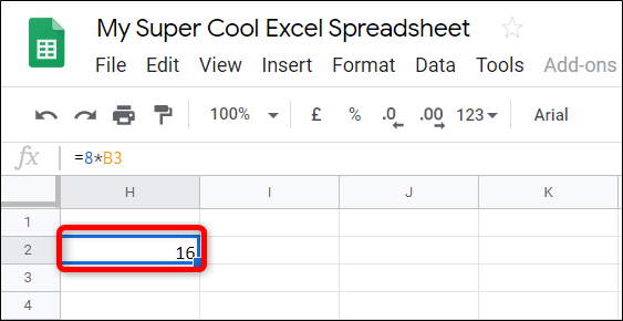
From a Google Sheets spreadsheet, click in the blank cell and type= *, replace and with the integer you want to multiply.

As before, you can reference other cells in the spreadsheet. Replace the number with the number of cells containing the integer.

After entering an integer or number of cells, press Enter to get the multiplication result.

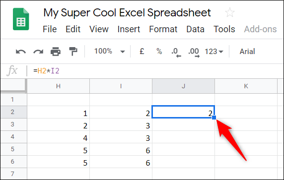
Tip : If you work with tables and want to multiply data from row 1 and row 2 into row 3, Google Sheets has a handy feature that applies formulas to the remaining cells. It will fill the remaining cells with formulas and results. Double click the small blue square and the rest of the table is filled with the result of multiplying two rows.

The kernel uses the ArrayFormula function

The next method uses the ArrayFormula function to display values returned from multiple rows or columns of the same size.

In the Google Sheets spreadsheet, click in the blank cell and type=ARRAYFORMULA( *, replace and with the two columns you want to multiply. It should look like this:

=ARRAYFORMULA(A:A*B:B)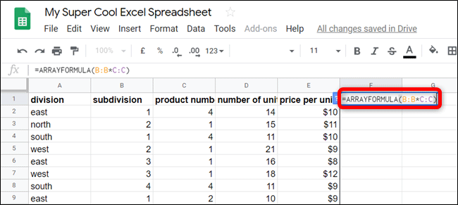

If the table has a heading in the first column, Sheets will display an error because it only takes numbers as parameters.

Therefore you should start with the first column containing numbers. For example, instead of A: A * B: B, you need to type A2: A * B2: B.

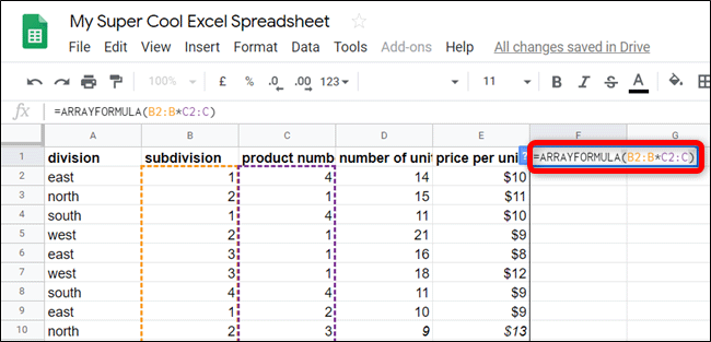
One thing to keep in mind is that when using this formula, empty cells with no numbers will display a result of 0. However, adding other data to the Sheets table will replace the number 0 with the actual result.

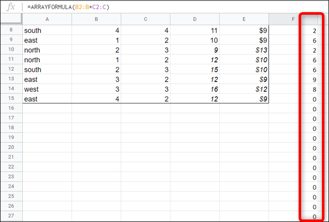
If you want to limit the number to 0 in the result, you should select a specific range when entering the formula. The new formula will be:

=ARRAYFORMULA(B2:B100*C2:C100)

With this formula, the spreadsheet uses only 100 cells as a reserve for all data entered later. You can edit the formula, delete any unused cells by changing 100 to smaller numbers.

When you need to multiply whole numbers, data from two cells, or the entire contents of a cell, Google Sheets provides several ways for you to calculate numbers.

I wish you successful implementation!