How to create Progress Bar in Excel, conditional progress bar

Creating a Progress Bar in Excel is not difficult, this tool is extremely simple but very useful in Excel and is used for many different purposes. With how to create a Progress Bar in Excel in this article, users will learn about one more feature in thousands of features that spreadsheets can make your work better.

Instructions for creating a Progress Bar in Excel

1. How to create Progress Bar in Excel 2019, 2016, 2013

Because Excel 2019, 2016 and 2013 versions have the same interface, here TipsMake will guide you to create Progress Bar in Excel on Excel 2016. Excel 2019 and Excel 2013 users can do the same.
==> Excel 2019 download link  here ==> Excel 2016 download
link   here ==> Excel 2013 download link  here

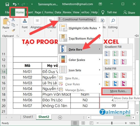
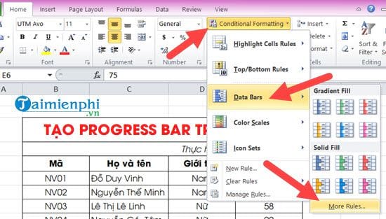
Step 1: On the Excel interface, go to Home > select Conditional Formatting > select Data Bars and select More Rules .
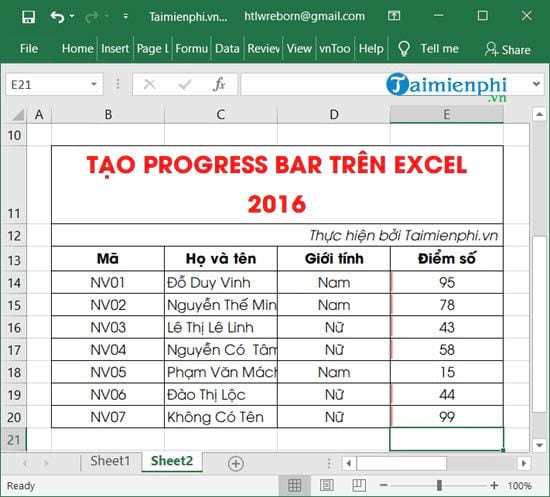
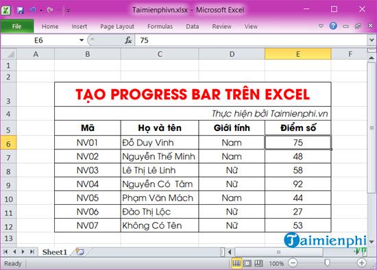
- Note that you must click on the cell where you want to create a Progress Bar in Excel first.

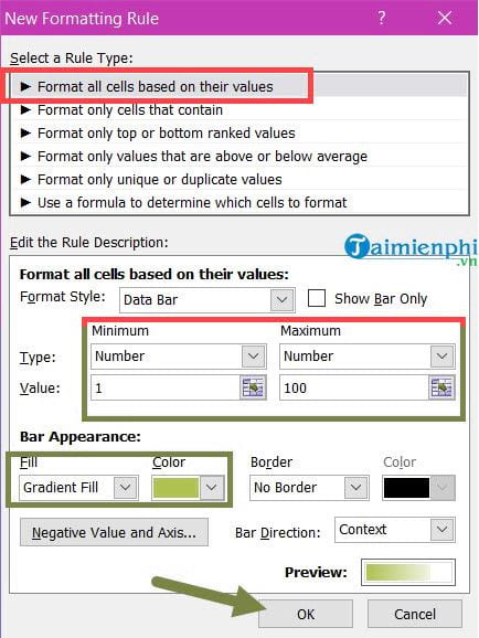
Step 2: In the New Formatting Rule section , select the following:

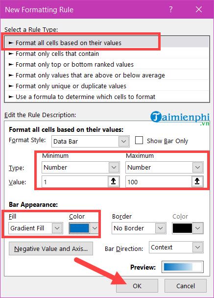
- Select a Rule Type : Select Format all cells based on their values.
- Edit the Rule Descripton : Here you set the Type to Number with Value Minimum as 1 and Maximum as 100. (Minimum is the minimum value of the number you enter and Maximum is the maximum, the system will base on that to display the Progress Bar).
- Bar Appearance : This part is up to you, you can choose the most pleasant color and then click OK.

Step 3: The first result is 95 corresponding to the displayed Progress Bar color column, now do the same for the remaining addresses.

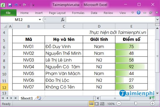
- You will see each cell value colored corresponding to the number we have specified (the highest is 100), that is how the Progress Bar is displayed.

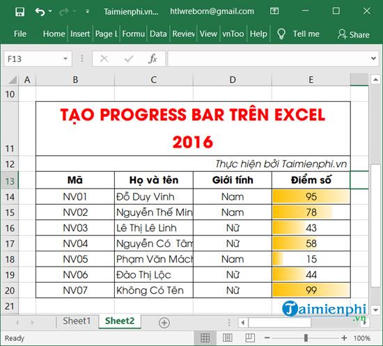
- Just change the values, the Progress Bars will also change accordingly, so we have completed how to create Progress Bar in Excel 2019, 2016 and Excel 2013.

2. How to create Progress Bar in Excel 2010, 2007

Similarly, now let's create a Progress Bar in Excel with the same example on Excel 2010, 2007.
==> Link  to download Excel 2010  here
==> Link  to download Excel 2007  here

Step 1: Open the Excel file, look at Home > select Conditional Formatting > select Data Bars and select More Rules .
- Note that you must click on the cell where you want to create a Progress Bar in Excel first.

Step 2: In the New Formatting Rule section , select as in the instructions for creating a Progress Bar in Excel 2016, 2013 to create a Progress Bar in Excel:

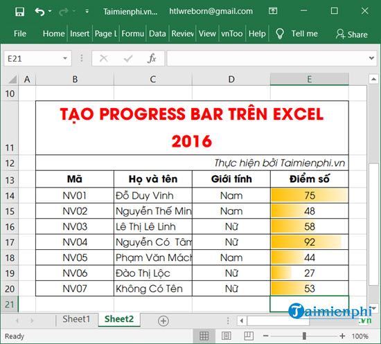
Step 3: The first result is 75 corresponding to the displayed Progress Bar color column, now repeat for all the above results.

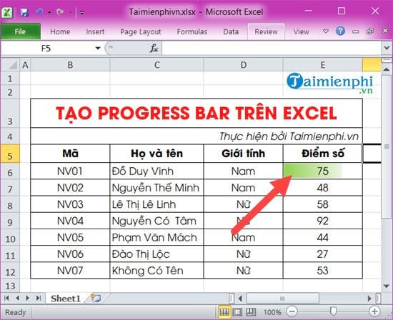
You will see each cell value is colored corresponding to the number we have specified (the highest is 100), that is how the Progress Bar is displayed.

So we have completed creating Progress Bar in Excel. Very simple and easy to do within 1 minute, right? Above are instructions on how to create Progress Bar in Excel 2019, 2016, 2013, 2010, 2007 by TipsMake. With the above instructions, creating Progress Bar will become simple and especially for new Excel users, this is a trick that cannot be ignored.

Above are instructions on how to create a Progress Bar in Excel 2016, 2013, 2010, 2007 from TipsMake. With the above instructions, creating a Progress Bar will become simple and especially for new Excel users, this is a trick that cannot be ignored.

In addition, when using Excel, don't forget to quickly familiarize yourself with  Excel shortcuts  and  how to line break in Excel. They will determine part of your operations as well as speed up your work progress.

Kareem Winters

Update 10 September 2024