CUMIPMT function - The function of calculating accrued interest in Excel

When you invest in a field, you always expect to get the greatest possible return. You want to calculate how much interest you have to pay when taking out a loan in case of accrualing such numbers. Compared to income? The following article is to use CUMIPMT function to calculate accrued interest. It helps you plan the lowest interest rate payment plan.

Introducing CUMIPMT function

Description: The function helps calculate the accrued interest to be paid from the beginning of the period to the end of a certain investment loan.

Syntax: CUMIPMT (rate, nper, pv, start_period, end_period, type) .

Inside:

- rate: The interest rate to be paid, it is a required parameter.

- nper: The number of periods payable during the borrowing period, which is a required parameter.

- pv: The present value of the loan, is the required parameter.

- start_period: The first payment period of the loan, is a required parameter.

- end_period: The last period of interest payment of the loan, which is the required parameter.

- type: The basis of determining the payment time, is a required parameter. There are 2 values, type = 0 => payment at the end of the period, type = 1 => payment at the beginning of the period.

Example: Give the following data table:

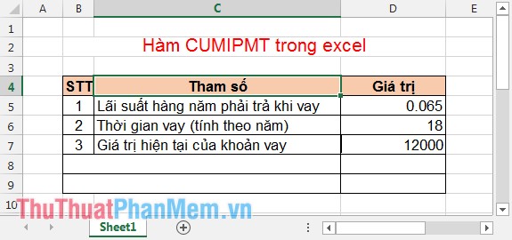
Calculate:

- Interest payable in the first month.

- Interest payable from 2nd to 15th month.

1. Interest paid in the first month

In the cell to calculate, enter the formula: = CUMIPMT (D5 / 12, D6 * 12, D7,1,1,0) .

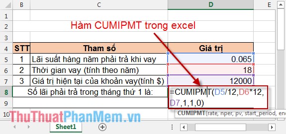
Result:

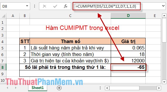
2. Interest paid from the 2nd to the 15th month

In the cell to calculate enter the formula: = CUMIPMT (D5 / 12, D6 * 12, D7,2,15,0) .

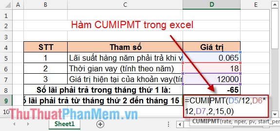
Result:

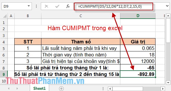
From February to November, total 14 months if paying interest by month => Total payable = 14 * 65 = 910 $ but accrued interest from February to 14 has to pay 892.89 $. Thus, accrued interest for many months saves you 1 money.

Above is an example and how to use CUMIPMT function to help you calculate the amount of interest to pay when borrowing investment capital.

Good luck!