6 Excel functions to find data quickly

1. FIND function

The FIND function in Excel returns the numeric position of a specified character or string (character string) within a larger string. This function is useful for exact text extraction, manipulation, and conditional formatting.

The syntax of the FIND function is:

FIND(search_text, text_to_search_in, [start_position])

Here, search_text is the character or substring you want to locate and text_to_search_in is the larger text string you want to search for. The start_position parameter specifies where in the string you want the function to start searching.

Note : Any parameters in square brackets are optional.

Here is an example of how the FIND function works:

=FIND("12345", "Order # 12345 - Completed")

The above formula will return 9, because the substring 12345 starts at that position.

6 Excel functions to find data quickly Picture 1

The FIND function is case sensitive. For example, if you search for the letter A in the substring apple, you will get an error.

If you want to find something that is case-insensitive, use the SEARCH function instead. This function has a similar syntax to the FIND function.

=SEARCH(search_text, text_to_search_in, [start_position])

2. SORT function

The SORT function can help you sort data in a range in ascending or descending order to make it easier to find specific data in your Excel spreadsheet.

The syntax of the SORT function is:

SORT(range_to_sort, [sort_index], [sort_order], [sort_by])

The range_to_sort parameter is the range you want to sort. Use the sort_index parameter to specify which column or row number to sort on within the range (default is 1).

The sort_order parameter specifies the order in which the list is sorted, where 1 is ascending and -1 is descending (the default is ascending). And sort_by specifies whether to sort by rows (FALSE) , which is the default, or by columns (TRUE) .

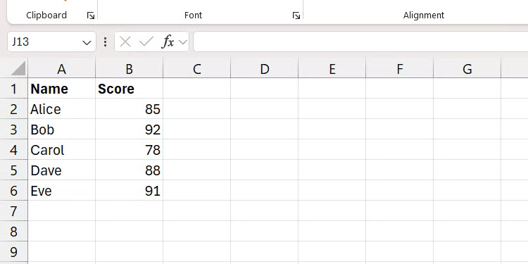
We will sort the range in the screenshot below based on the second column and in descending order.

6 Excel functions to find data quickly Picture 2

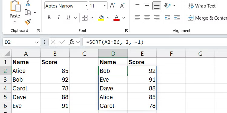
Here's how the formula will look in Excel:

=SORT(A2:B6, 2, -1)

The range will now be sorted in descending order.

6 Excel functions to find data quickly Picture 3

3. FILTER function

The FILTER function evaluates a range of data based on a condition and returns only rows and columns that meet the condition.

The syntax of the FILTER function is:

FILTER(range_to_filter, condition, [value_if_empty])

The range_to_filter parameter is the array or range of cells you want to filter. The condition parameter is the criteria that determines what content will be returned in the filtered results. The value_if_empty parameter specifies what content will be returned if no content meets the condition.

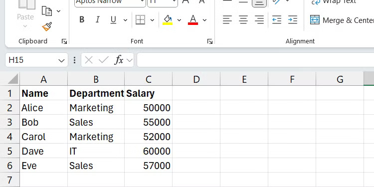
We will filter the scope in the screenshot below to only show employees in the Sales department .

6 Excel functions to find data quickly Picture 4

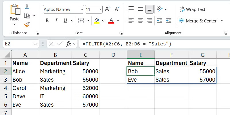
Here is an image of the formula in action:

=FILTER(A2:C6, B2:B6 = "Sales")

Now, you should only see rows and columns that meet the specified criteria.

6 Excel functions to find data quickly Picture 5

4. INDEX function

If you want to get the value of a specific cell in a range of data, you can use the INDEX function. You just need to specify the row and column where the value will be located.

The syntax of the INDEX function is:

INDEX(range_to_search, row_to_search_in, [column_to_search_in])

The range_to_search parameter is the range you will get the value from. row_to_search_in and column_to_search_in are the row and column numbers the value falls within (think of them as coordinates).

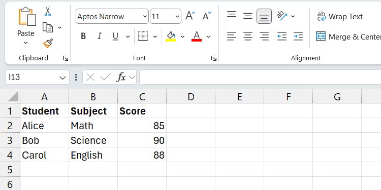
For example, in the screenshot below, we will take the Score ( C4 ) that Alice got in her English test.

The range in Excel displays students' test scores in different subjects.
The formula looks like this:

=INDEX(A1:C4, 4, 3)

This formula will return 88 because that is the score Alice got on her English test.

6 Excel functions to find data quickly Picture 6

5. MATCH function

The MATCH function in Excel searches a range of data for a specified value and then returns its relative position. You can then use the returned value with functions like INDEX to retrieve and manipulate the data dynamically.

The syntax of the MATCH function is:

MATCH(value_to_search, range_to_search_in, [match_type])

Here, value_to_search is the value you want to find and range_to_search_in is the range in which you are searching for that value.

The match_type parameter specifies the type of match to use. Here are the types you can use:

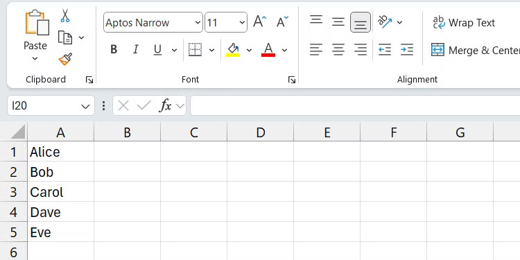
In the example, we will use the MATCH function to find Carol's position in the range, requiring that it be an exact match.

6 Excel functions to find data quickly Picture 7

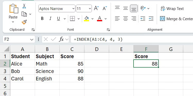
Here is what the function would look like in Excel:

=MATCH("Carol", A2:A6, 0)

After running the above formula, the function will return 3 because Carol's exact match is the third item in the range.

6 Excel functions to find data quickly Picture 8

6. Find XLOOKUP

With the XLOOKUP function, you specify a value to look up in one range and then retrieve the corresponding value from another range. Unlike the HLOOKUP and VLOOKUP functions, XLOOKUP allows you to look up in any direction, making it more flexible to look up data in a spreadsheet.

The syntax of the XLOOKUP function is:

XLOOKUP(value_to_look_up, range_to_check, range_to_return, [if_value_not_found], [match_type], [search_mode])

In this syntax, value_to_look_up is the value you are looking for, range_to_check is the range from which the value you want to retrieve is, and range_to_return is where the corresponding value of the lookup value will come from. You only need to specify these 3 parameters for the function to work, so these are the only ones we will focus on.

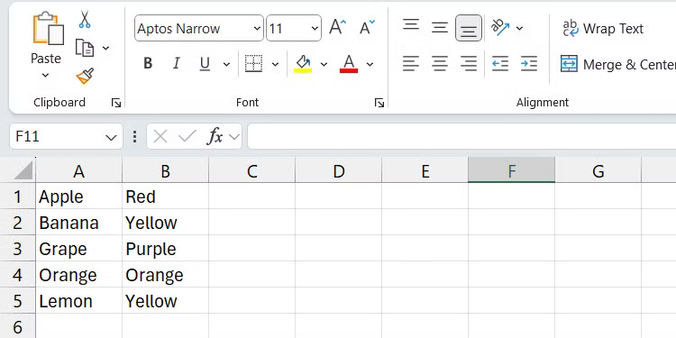
Let's clarify this with an example based on the screenshot below. The example wants to search for Banana (A2) and return its color from the corresponding column (B) .

6 Excel functions to find data quickly Picture 9

Here's how the formula would look in Excel:

=XLOOKUP("Banana", A:A, B:B)

Running this formula will return Yellow (B2) , the corresponding value based on the lookup of the Banana value.

6 Excel functions to find data quickly Picture 10

Mastering these six Excel functions - FIND, SORT, FILTER, INDEX, MATCH, and XLOOKUP - will help you quickly locate, sort, and extract information from large data sets. This can dramatically improve your Excel productivity and your ability to analyze data effectively.

David Pac

Update 09 December 2024