Comparison functions in Excel - How to use comparison functions and examples using comparison functions

With a large amount of data, you want to check for duplicates by checking normally, it is really hard. In this article, I introduce you to the Comparison Functions in Excel, with practical examples to help you easily visualize.

1. Use the Exact function to compare data

Description

The Exact function compares two text strings, returning True if the two strings match, and returning False if the two data strings are different. Note The Exact function is case-sensitive.

Syntax

EXACT (Text1, Text2)

Where: Text1, Text2 are two text strings to be compared, are two required parameters.

Attention

- The Exact function is case sensitive, but it does not distinguish format.

For example

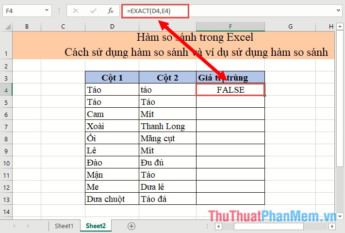
Compare the corresponding data in rows between column 1 and column 2. In the cell to compare enter the formula: EXACT (D4, E4)

Pressing Enter results returns a False value, which means the two values ​​do not match because of the first and lowercase letters:

Similarly copying the formula for the remaining values ​​results:

However, with this function, you cannot compare a value in column 1 with all the data in column 2 to find a duplicate. With this function you can only compare rows between themselves.

2. Use the Countif intermediate function to compare data

To overcome the situation in example 1, you can use the Countif function as an intermediary to compare the values ​​in column 1 against the values ​​in column 2.

Description of the Countif function

- Countif function counts the number of cells that meet certain conditions in the selected data range.

Syntax

COUNTIF (Range, Criteria)

Inside:

- Range: The data area containing the data to be counted, is a required parameter.

- Criteria: The condition used to count data, is a required parameter

For example

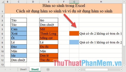
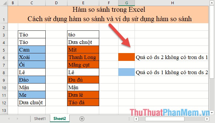
Compare data between 2 columns, highlight values ​​not in column 1 but in column 2 and vice versa.

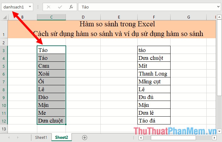
Step 1: Name the data columns:

Select the entire column 1 data into the address bar enter listname1 -> press Enter.

Step 2: Similar to the name of column 2, then the names of 2 data columns are displayed:

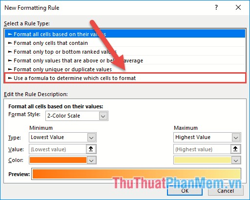
Step 3: Select the whole list 1 -> go to Home tab -> Conditional Formatting -> New Rule .

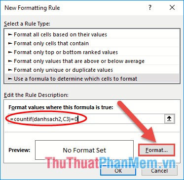
Step 4: A dialog box appears, select Use a formula to determine which cells to format:

Step 5: Enter the formula = COUNTIF (list2, C3) = 0 then click Format:

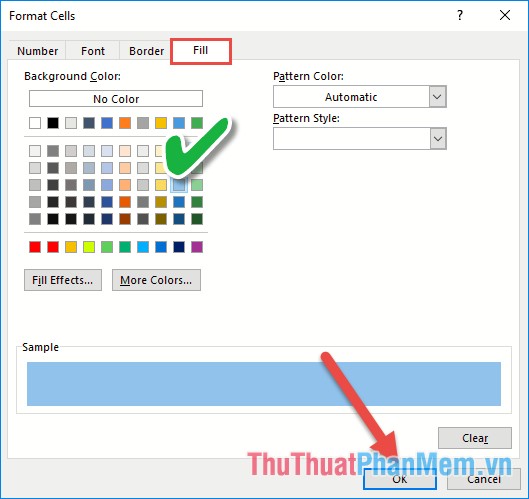
Step 6: The Format Cells dialog box appears, click the Fill tab -> select the color marking the fruit is not in the list 2 -> click OK:

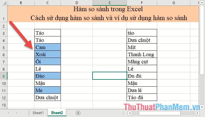
Step 7: Next, click OK to close the resulting fruits dialog box in List 1, which is not in List 2, which is colored to distinguish:

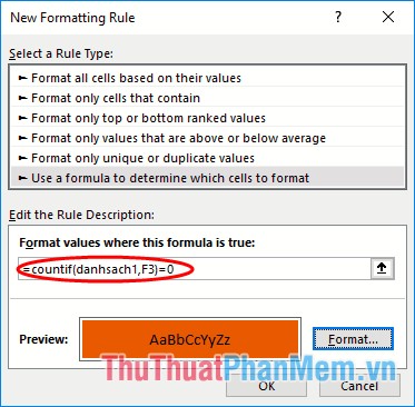
Step 8: Similar to the list 2 you do the same, but only differ from the formula: = COUNTIF (list2, F3) = 0 , it will color the cell with a value of 0 (not the same)

As a result, you have compared 2 columns of data and can add notes for readers to easily visualize:

Above is an instruction on how to use EXACT function , application COUNTIF function  to compare data in Excel. Good luck!