How to combine Index and Match functions in Excel

The search function in Excel is part of the basic Excel function group and there are many different options for you to find the value you need in the table, such as using the Excel Vlookup function or the Hlookup function. However, the two search functions will only search for values ​​in rows or columns, in one direction, without looking for values ​​on both rows and columns.

In this case, we should combine the Index and Match functions to get the values ​​in the rows and columns, easier to do to replace the search function Vlookup or Hlookup. The following article will guide you how to combine 2 Index and Match functions in Excel.

1. Use the VLOOKUP function to join two Excel tables together
2. How to combine Sumif and Vlookup functions in Excel?
3. How to combine 2 columns of First and Last Names in Excel does not lose content
4. 2 ways to separate first and last name information in Microsoft Excel?

Instructions for combining the Index and Match functions in Excel

1. Index function in Excel

The Index function has 2 forms: the array function and the reference index.

The array function returns the value of a data cell with the row and column index searched. The network function syntax is Index (Array, Row_num, [column_num]). Inside:

1. Array: Array of referenced data or an array constant.
2. Row_num: The row containing the value to retrieve.
3. Column_num: Column containing the value to retrieve.

The reference index function returns the value of a cell with the row and column indexes being searched. The syntax of the function of the reference form is INDEX (Reference, Row_num, [Column_num], [Area_num], in which:

1. Reference: The reference area contains the value to search.
2. Row_num: The row index containing the value to search.
3. Column_num: The column index containing the value to search.
4. Area_num: Number of regions returned, left blank is 1 default.

Learn more about using the Index function in the article How to use the Index function in Excel.

2. Match function in Excel

The Match function returns the ordinal number of the value to find in the table. The structure of the Match function is = MATCH (Lookup_Value, Lookup_array, [Match_type]). Inside:

1. Lookup_Value: The value to search.
2. Lookup_array: Array contains the value to look for.
3. Match_type: Search type. There are 3 types of searches:
   1. Search for values ​​less than what to look for when match_type = 1.
   2. Search for the value equal to the value to search when match_type = 0.
   3. Search for a value greater than the value to search when match_type = -1.

How to use the Match function you read in the article How to use the Match function in Excel.

3. Combining the Match function with the Index function

We have the data sheet as shown below.

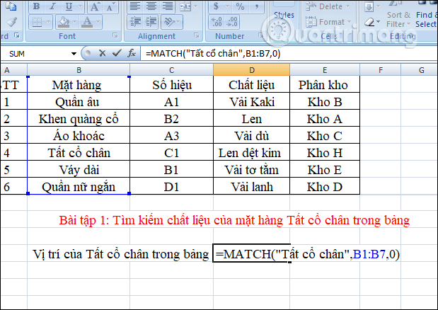
Exercise 1: Searching for the material of the ankle socks in the table (Find right to left)

According to the table we see the location of the ankle socks is at No. 4 and to close to see the material of the ankle socks is knitted wool. So we will look at the Material column and look to row 5 to get the result.

Step 1:

First of all we will find the item in the ankles located anywhere in the table. Enter the formula = MATCH ("Socks", B1: B7,0) and press Enter. Inside:

1. Ankles: Is the value to find the right position.
2. B1: B7: Search area for values, here is the Items column.
3. 0: Find the exact value.

The result will be 5, meaning that the ankles are at the 5th row in the table .

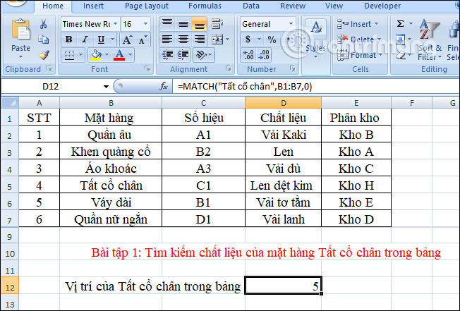
Step 2:

Now we will find the value in the Material column corresponding to the value in line 5 , which will produce the material for the ankle socks.

The formula that combines the INDEX function with the MATCH function is = INDEX (the column to look up the value, (MATCH (the value to look up, the column that contains the value, 0)) .

Applied to Exercise 1, you can also replace the MATCH cluster (the value used to look up, the column containing the value, 0)) = 5, the order of the value used to look up.

Enter the formula as = INDEX (D1: D7,5) and press Enter. In which D1: D7 is the column containing the value to look up.

The result will be Knitted Wool.

The general formula that combines INDEX with MATCH when applying to exercise 1 is = INDEX (D1: D7, MATCH ("Socks", B1: B7,0)) and press Enter.

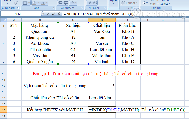
The results also showed that knitted wool corresponds to ankle socks.

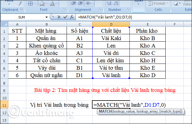
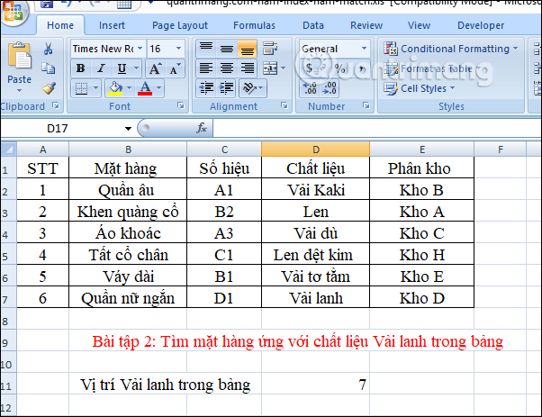
Exercise 2: Finding items corresponding to Linen in the table (Find from left to right)

Step 1:

First of all we need to find the position of the Linen in the Material column . Enter the formula = MATCH ('Linen', D1: D7,0) and press Enter. Inside:

1. Linen: Need to find a position for this value.
2. D1: D7: The data area contains the value to find the position.
3. 0: Find exactly this value.

Output 7, Linen is in line 7 in the Material column.

Step 2:

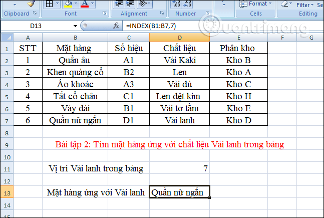
Combined with the INDEX function, we have the formula = INDEX (B1: B7,7) and press Enter.

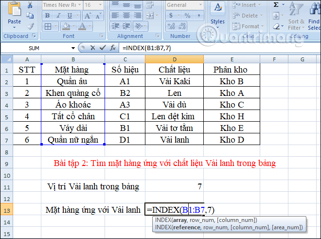
The result will show Short pants for women as per the table.

We will combine INDEX with MATCH in the same input formula = INDEX (B1: B7, MATCH ('Linen', D1: D7,0)) and press Enter.

The results also showed for short pants.

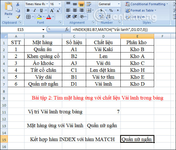
Thus, when combining INDEX function with Excel function, we will search for values ​​in both directions from left to right or right to left. With the VLOOKUP function, we can only look up data from left to right.

Read the exercise of combining INDEX and MATCH with the following link.

1. Download the INDEX function assignment with the MATCH function

I wish you successful implementation!