How to master numerical data in Google Sheets with the AVERAGE function

 The following article will show you how they work.

1. AVERAGE function

The AVERAGE function calculates the average value of a range of numbers by adding them up and dividing by the number of numbers. The following is the syntax of the AVERAGE function:

=AVERAGE(range)

Where range represents the range of cells for which you want to calculate the average.

Example of AVERAGE calculation

Suppose you want to calculate the average value of monthly utility costs and the data is in two columns. The utility name is in cells A2:A5 of column A, while the cost is in cells B2:B5 of column B.

To find your average monthly utility costs, use the formula:

=AVERAGE(B2:B5)

How to master numerical data in Google Sheets with the AVERAGE function Picture 1

In the case example, the average monthly utility cost is $128.75.

2. AVERAGEA function

The AVERAGEA function calculates the average value of a range, considering both numbers and text. However, the text is considered zero during the calculation. This function can be useful when you want to calculate the mean for a data set that includes non-numeric content.

The following is the syntax for the AVERAGEA function:

=AVERAGEA(range)

Where range represents the range of cells you want to include in the average.

Example of AVERAGEA calculation

Imagine you just learned some task management tips and decided to create a to-do list. However, when tracking the number of tasks completed each day, you did not mark some tasks as completed and instead entered N/A.

In this example, let's assume the number of tasks you completed are in cells B2:B6 . To calculate the average, use the formula:

=AVERAGEA(B2:B6)

How to master numerical data in Google Sheets with the AVERAGE function Picture 2

Because the example has "N/A" in cell B4, this value is considered zero during the calculation.

3. DAVERAGE function

The DAVERAGE function calculates the average of the values ​​in a specified column in the database, but only for those rows that meet the given criteria. The syntax of the DAVERAGE function is:

=DAVERAGE(database, field, criteria)

Where database represents the range of cells that make up the database, field is the column to calculate the average value and criteria is the range containing the filtering conditions for which rows will include the average value.

Example of DAVERAGE calculation

Let's say you're tracking the average time spent watching TV, but you only want to include days where you watch more than 2 hours. The days you watched TV are in cells A1:A5 and the hours spent watching TV are in cells B2:B6.

Additionally, let's say you have criteria data in column D. Since we're focusing on days when you watched TV for more than 2 hours, you would have to put Hours in cell D2 and >2 (greater than 2) in cell D3 .

Finally, to calculate the average time you spend watching TV over 2 hours during the week, you would use the formula:

=DAVERAGE(A1:B6, "Hours", D2:D3)

How to master numerical data in Google Sheets with the AVERAGE function Picture 3

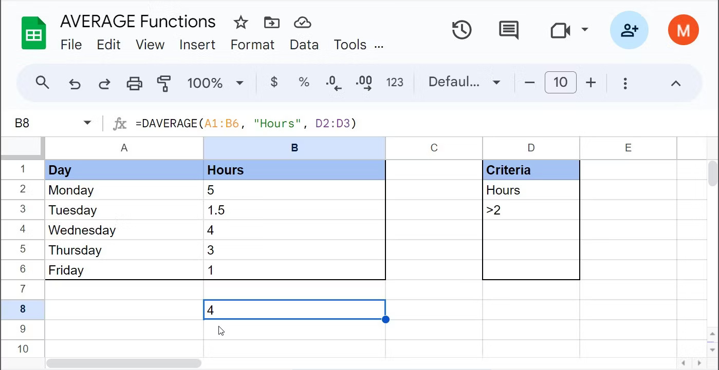
In the example case, there are 3 days a week of watching TV for more than 2 hours, an average of 4 hours/day.

4. AVERAGEIF function

The AVERAGEIF function calculates the average of the values ​​in cells that meet a specified condition. The following is the syntax for the AVERAGEIF function:

=AVERAGEIF(range, criteria, [average_range])

Where range represents the cells you want to evaluate against the criteria, criteria is the condition that determines which cells will be included in the average, and average_range (optional) is the actual range of cells to calculate the average .

Example of the AVERAGEIF calculation

Let's say you want to find the average weekly fuel costs only in cases where you spend more than $50. Suppose you have fuel costs in cells B2:B6 .

To get the average of the values ​​above $50, use the formula:

=AVERAGEIF(B2:B6, ">50")

How to master numerical data in Google Sheets with the AVERAGE function Picture 4

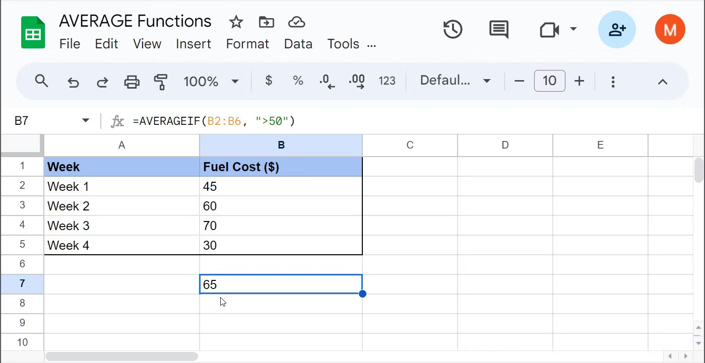
In the example case, the average cost for all values ​​above 50 USD is 65 USD.

5. AVERAGEIFS function

The AVERAGEIFS function is similar to AVERAGEIF but allows multiple criteria. The syntax of the AVERAGEIFS function is:

=AVERAGEIFS(average_range, criteria_range1, criteria1, [criteria_range2, criteria2], …)

Where average_range is the range of cells to calculate the average, criteria_range1 is the range you want to evaluate according to the first criterion, criteria1 is the first condition that determines which cells will be included in the average value and can be further specified. other scopes and criteria.

AVERAGEIFS calculation example

Let's say you're tracking sales data for products in many different cities. The cities are in cells A2:A6 , the products are in cells B2:B6 , the number of products sold is in cells C2:C6 , and the months in which the products were sold are in cells D2:D6 .

Let's say you want to find average sales within the city range of New York and the product is Gaming PC. In this case, the formula will be:

=AVERAGEIFS(C2:C6, A2:A6, "New York", B2:B6, "Gaming PC")

How to master numerical data in Google Sheets with the AVERAGE function Picture 5

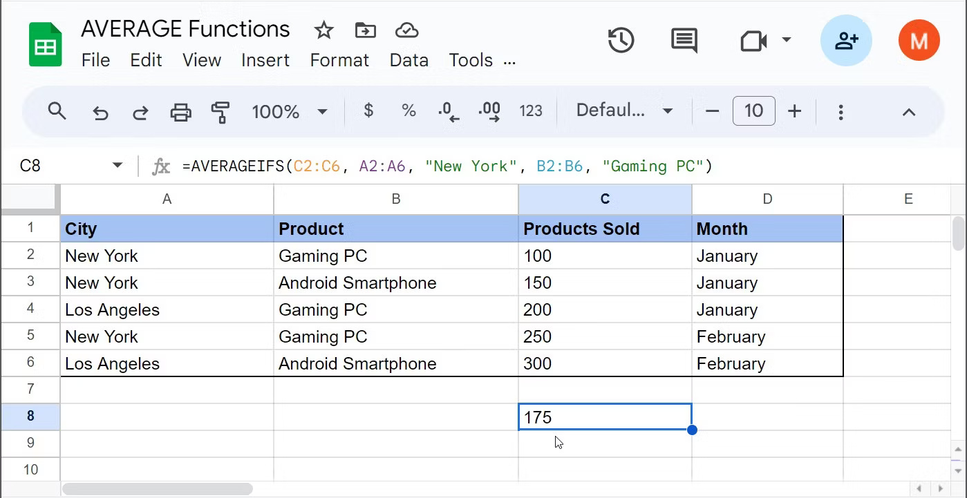
This function will return the average sales for New York and Gaming PC over different periods. In the case example, the average value is 175 gaming computers sold in New York.

6. AVERAGE.WEIGHTED function

The AVERAGE.WEIGHTED function calculates a weighted average, useful when some values ​​in a data set contribute more to the mean than others. This function considers both the values ​​and their respective weights in the calculation. A common example of this is calculating GPA.

The following is the syntax of the AVERAGE.WEIGHTED function:

=AVERAGE.WEIGHTED(values, weights)

Where values ​​denotes the range of cells containing the values ​​to calculate the average, and weights denotes the range of cells containing the corresponding weights for the values.

Example calculation of AVERAGE.WEIGHTED

Imagine you are a student who has just learned tips on how to study effectively. Now, you want to calculate a weighted average of the study hours of different subjects, with some subjects being more important than others. Subjects are in cells A2:A6 , class hours are in cells B2:B6 , and weights are in cells C2:C6.

The weight values ​​are 1-4, where 1 represents "less important" and 4 represents "most important."

To calculate a weighted average of study hours based on the importance of each subject, use:

=AVERAGE.WEIGHTED(B2:B6, C2:C6)

This formula multiplies the study hours by their respective weights, adds these values, then divides by the total weight to get the overall weighted average study time.

How to master numerical data in Google Sheets with the AVERAGE function Picture 6

In the example case, the weighted average study time is 7.5 hours. This means that, when considering the importance (weight) of each subject, the average study time is equivalent to 7.5 hours per subject.

Here's how AVERAGE.WEIGHTED can help determine whether your current study schedule fits your study priorities.

1. Math : 10 hours (above average of 7.5 hours). This means spending more time than average, in accordance with the priority/weight of the subject.
2. Science : 8 hours (higher than 7.5 hours). This is slightly higher than the weighted average and is consistent with the importance of the subject.
3. History : 5 hours (less than 7.5 hours). This is less than average, which is acceptable because this subject has a lower priority/weight.
4. Literature : 4 hours (much less than 7.5 hours). This is significantly less than the average, consistent with the subject's lower priority.
5. Language : 6 hours (less than 7.5 hours). This number is a bit lower but still quite close to the weighted average, which should be fine based on the subject's weight.

AVERAGE functions provide a simple yet powerful means of processing data. By using them effectively, you can perform data analysis in Google Sheets seamlessly and draw meaningful conclusions from complex data sets.

David Pac

Update 27 August 2024