8 How to delete blank rows in ExcelHow to delete blank rows in Excel

They will make certain things like navigating around our data much more difficult.

But the good news is that there are many ways to get rid of these unwanted rows and it can be quite easy to do so.

In this post, we will look at 9 ways to remove blank rows from our Excel data.

Delete empty rows manually

The first method is the manual way.

Don't worry, we'll get to easier methods later. But if we only have a few rows then the manual way might be faster.

8 How to delete blank rows in ExcelHow to delete blank rows in Excel Picture 1

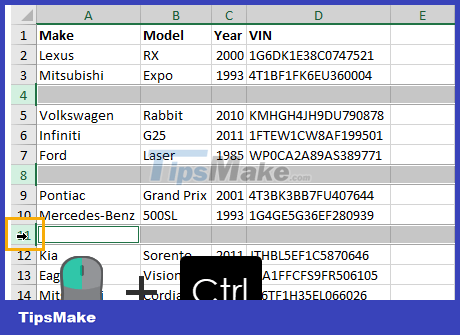
Select the blank rows we want to delete. Hold down  the Ctrl key  and click a row to select it.

8 How to delete blank rows in ExcelHow to delete blank rows in Excel Picture 2

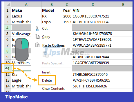
Once the rows we want to delete are selected then we can  right click and select Delete  from the menu.

8 How to delete blank rows in ExcelHow to delete blank rows in Excel Picture 3

We can also delete rows using the ribbon command. Go to the Home tab ➜ click the Delete command  ➜ and then select Delete Sheet Rows  .

8 How to delete blank rows in ExcelHow to delete blank rows in Excel Picture 4

There is also a very handy keyboard shortcut to delete rows (columns or cells). Press  Ctrl  +  –  on the keyboard.

That's it! Our empty row is now gone.

Delete empty rows using special move to

Manually selecting and deleting rows is OK if we only have a few rows to delete.

What if there are many empty rows spread across our data? Manual selection would be a pain!

Don't worry, there's a command in Excel that selects all the blank cells for us.

8 How to delete blank rows in ExcelHow to delete blank rows in Excel Picture 5

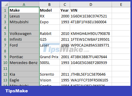
First, we need to select a column of data that includes all blank rows. The easiest way to do this is to select the first cell (A1 in this example), then hold down the  Shift key  and select the last cell (A14 in this example).

8 How to delete blank rows in ExcelHow to delete blank rows in Excel Picture 6

We can now use the  Go To Special command  to select only empty cells. Go to Home tab  ➜ press Find & Select command ➜ select Go To Special  from the menu.

8 How to delete blank rows in ExcelHow to delete blank rows in Excel Picture 7

There's also a handy shortcut for the Go To menu  . Press  Ctrl  +  G to open the Go To menu , then click the Special button to open the Go To Special menu  .

8 How to delete blank rows in ExcelHow to delete blank rows in Excel Picture 8

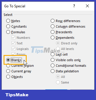
Whether we open the Go To menu and then click Special   or we go directly to the Go To Special menu , we will arrive at the same Go To Special menu  .

Now all we need to do is select  Blanks  from the options and press the  OK button  . This will select only empty cells from our initial column selection.

8 How to delete blank rows in ExcelHow to delete blank rows in Excel Picture 9

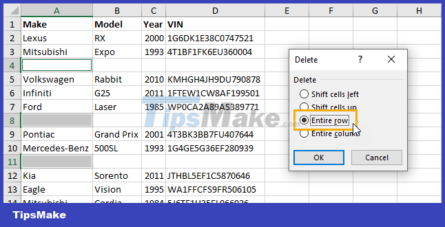
Now we need to delete those selected rows.

1. Use any of the row deletion methods from the Delete Blank Rows Manually section  .
   1. Right-click ➜ Delete
   2. Home Tab ➜  Delete  ➜  Delete Sheet Rows
   3. Shortcut key Ctrl +  –
2. In the Delete menu  , select Entire row  and press the  OK button  .

Like magic, we can find and delete hundreds of blank rows in our data within seconds. This is especially good when we have a lot of empty rows scattered across a long data set.

Delete empty rows using the find command

This method will be very similar to the  Delete Empty Rows method above using the  Special method  . The only difference is that we will select our empty cells using the Find command  .

Like before, we need to select a column in our data.

8 How to delete blank rows in ExcelHow to delete blank rows in Excel Picture 10

Go to the  Home tab ➜ press the Find & Select command  ➜ select Find from the menu.

8 How to delete blank rows in ExcelHow to delete blank rows in Excel Picture 11

There is also a keyboard shortcut that we can use to open the Find menu . Press  Ctrl  +  F  on the keyboard.

8 How to delete blank rows in ExcelHow to delete blank rows in Excel Picture 12

Either way, this opens the Find & Replace menu for us.

1. Expand the Advanced options   in the Find menu.
2. Leave the Find what input box blank .
3. Select the Match entire cell contents option .
4. Within select Sheet
5. Look select Values
6. Press the FInd All button to return all blank cells.

8 How to delete blank rows in ExcelHow to delete blank rows in Excel Picture 13

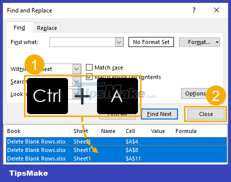
This will display a list of all empty cells found in the selected range at the bottom of the Find menu.

We can select all of them by pressing  Ctrl  +  A . We can then close the Find menu by pressing the Close button  . Now we can delete all the empty cells like before.

Remove empty rows using a filter

We can also use a filter to find empty rows and remove them from our data.

8 How to delete blank rows in ExcelHow to delete blank rows in Excel Picture 14

First, we need to add filters to our data.

1. Select the entire range of data including blank rows.
2. Go to the Data tab  .
3. Click the Filter button  in the Sort & Filter section.

8 How to delete blank rows in ExcelHow to delete blank rows in Excel Picture 15

We can also add a filter to a range of cells using the keyboard shortcut  Ctrl  +  Shift  +  L.

8 How to delete blank rows in ExcelHow to delete blank rows in Excel Picture 16

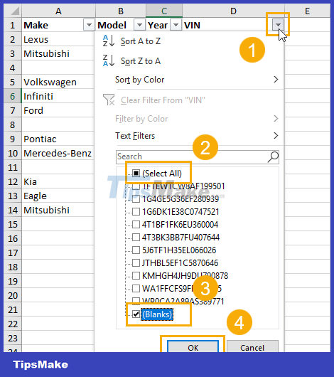
This will add sorting and filtering toggles for each column header, and we can now use them to filter out blanks.

1. Click filter toggle on one of the columns.
2. Use the Select All toggle to deselect all items.
3. Check out the Blanks  .
4. Press the  OK button  .

8 How to delete blank rows in ExcelHow to delete blank rows in Excel Picture 17

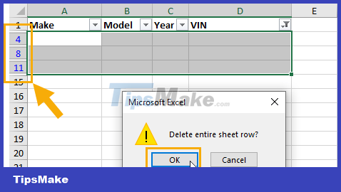
When our data is filtered, row numbers appear in blue and the filtered rows are missing numbers.

Now we can select these empty rows with blue row numbering and delete them using any manual method.

Then we can press the  OK button when Excel asks us if we want to Delete entire sheet row  .

Once we remove the filters, all our data will still be there but no empty rows!

8 How to delete blank rows in ExcelHow to delete blank rows in Excel Picture 18

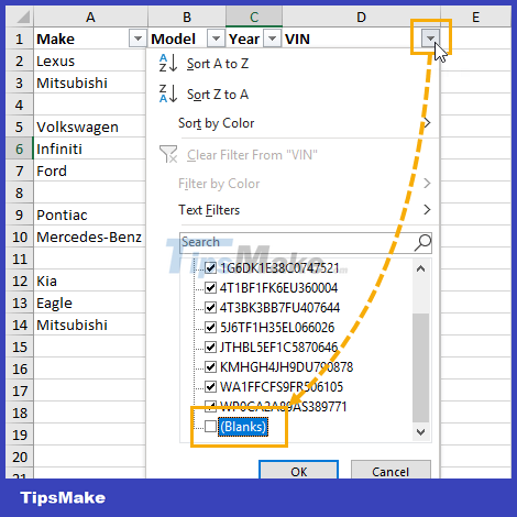
We can use filters in a slightly different way to remove empty rows. This time we will filter out the blanks. Click filter toggle on one of the columns ➜ uncheck Blanks   ➜ press  OK button  .

8 How to delete blank rows in ExcelHow to delete blank rows in Excel Picture 19

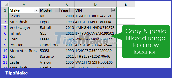
Now all our blank rows are hidden and we can copy and paste our data into a new location without all the blank rows.

Remove empty rows using advanced filters

Similar to the filter method, we can use the Advanced Filters option to get a copy of our data minus any blank rows.

8 How to delete blank rows in ExcelHow to delete blank rows in Excel Picture 20

To use the Advanced Filters feature , we will need to do a bit of setup work.

1. We need to set the filter criteria range. We will only be filtering based on one column, so we need a column header from our data (in this example, F1). Below the column header, we need our criteria (in this example F2), which we need to enter  =""in this cell as our criteria.
2. Select the data range to filter.
3. Go to the Data tab .
4. Select Advanced in the Sort & Filter section .

8 How to delete blank rows in ExcelHow to delete blank rows in Excel Picture 21

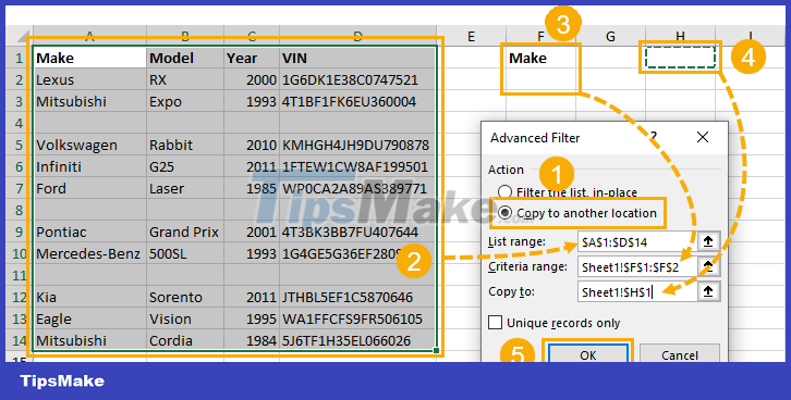
Now we need to configure the Advanced Filter menu.

1. Select Copy to another location  .
2. Select the range of data to be filtered. This will be populated if the range was selected before opening the advanced filter menu.
3. Add criteria to the Criteria range  (F1:F2 in this example).
4. Select a location in the worksheet to copy the filtered data.
5. Press the OK button .

Now we get a copy of our data in the new location without empty cells.

Remove empty rows using the filter function

If we're using Excel Online or Excel for Office 365, then we can use one of the new dynamic array functions to filter out our blank rows.

Actually, there is a  dynamic array FILTER function  that we can use.

FILTER function syntax

= FILTER ( Array, Include, [Empty] )

1. Array  is the range of data to filter.
2. Include  is a logical expression that indicates what to include in the filtered results.
3. Empty  is the result displayed if no results are found based on the Include argument.

FILTER function to filter empty spaces

8 How to delete blank rows in ExcelHow to delete blank rows in Excel Picture 22

= FILTER ( CarData, CarData[Make]<>"" )

The above function only needs to enter one cell and the results will overflow to the remaining cells as needed. The function will filter  CarData  on the  Make column  and filter out any blanks.

It's easy and the great part is that it's dynamic. Because our data is in an Excel table, when we add new data to the  CarData table  , it will appear in our filtered results.

Remove empty rows by sorting

8 How to delete blank rows in ExcelHow to delete blank rows in Excel Picture 23

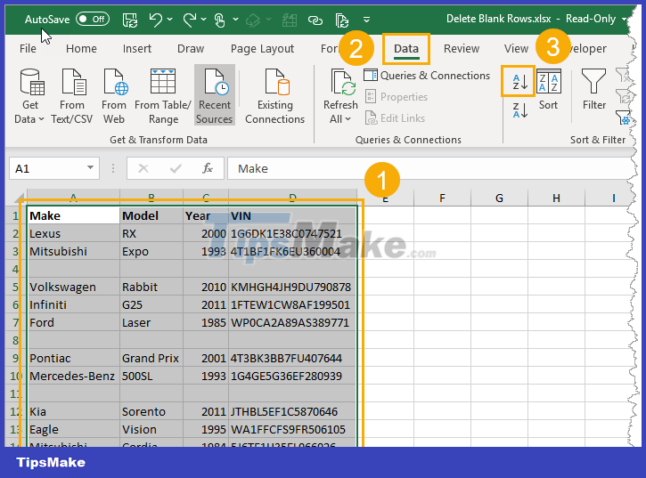
In addition to all the filtering techniques, we can sort our data to get all the empty rows.

1. Select data range.
2. Go to the Data tab  .
3. Press the sort command. Ascending or descending order will work.

8 How to delete blank rows in ExcelHow to delete blank rows in Excel Picture 24

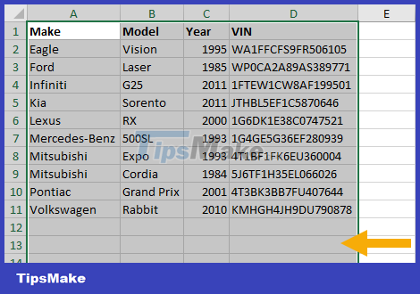
Now all our empty rows will appear at the bottom and we can ignore them.

If we need the initial sort order of the data, we can add an index column before sorting. We can then sort to get the empty rows at the bottom and delete them. We then sort our data back to its original order based on the index column.

Delete empty rows using Power Query

Power can easily remove blank rows in our data.

This is great in that we keep getting updated data with gaps in it and need to factor this into our data preparation steps.

8 How to delete blank rows in ExcelHow to delete blank rows in Excel Picture 25

Once our data is inside the source query editor, we can easily delete our empty data. Note, they appear as  null values  ​​inside the editor.

1. Go to the Home tab  in the source query editor.
2. Click the Remove Rows button  .
3. Select the Remove Blank Rows option  from the menu.

= Table.SelectRows(#"Changed Type", each not List.IsEmpty(List.RemoveMatchingItems(Record.FieldValues(_), {"", null})))

This will generate the M code above using the  Table.SelectRows function  to select non-null rows. This will only remove rows where the entire record has a null value.

8 How to delete blank rows in ExcelHow to delete blank rows in Excel Picture 26

We can also get the same result by filtering out null values   ​​in our data. Right-click any sort and filter toggle, then uncheck the null  value   and press the  OK button  .

= Table.SelectRows(#'Changed Type', each ([Model] <> null))

The source query will again generate a step with the Table.SelectRows function, which returns non-empty values ​​in a specific column.

Micah Soto

Update 01 October 2023