How to compare data on 2 Excel columns

Excel functions are all basic functions on Excel, such as COUNTIF functions. The COUNTIF function is used to count cells that meet certain conditions within the range of conditions specified. With COUNTIF function, users can compare data between 2 columns to find different data. The following article will show you how to compare data between 2 columns with the COUNTIF function.

1. How to combine Sumif and Vlookup functions in Excel
2. How to automatically display names when entering code in Excel
3. How to use Vlookup function in Excel

Instructions for using COUNTIF Excel function

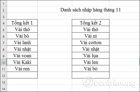
For example, we have a list of import items on Excel as below.

How to compare data on 2 Excel columns Picture 1

Step 1:

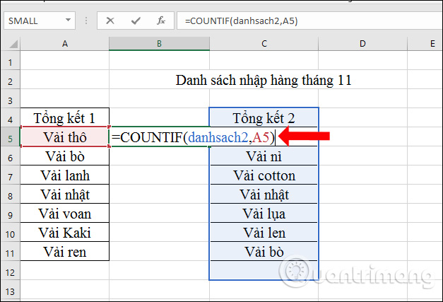
First, black out the data in column 1 (Summarize 1) , remove the title and place your cursor in the Name Box above to write any unsigned name, write as shown and press Enter.

How to compare data on 2 Excel columns Picture 2

Step 2:

Continue to do the same with column 2 (Summary 2).

How to compare data on 2 Excel columns Picture 3

Step 3:

In the column between the two columns of data, click in the empty box above and then enter the formula = COUNTIF (danhsach2, A5) and press Enter. We will begin to compare the data of the list column1 with the name column column2, starting from cell A5 of list1.

Note that depending on the Excel version, we use the mark; or, in the formula. If you report an error when entering, please change it again.

How to compare data on 2 Excel columns Picture 4

Step 4:

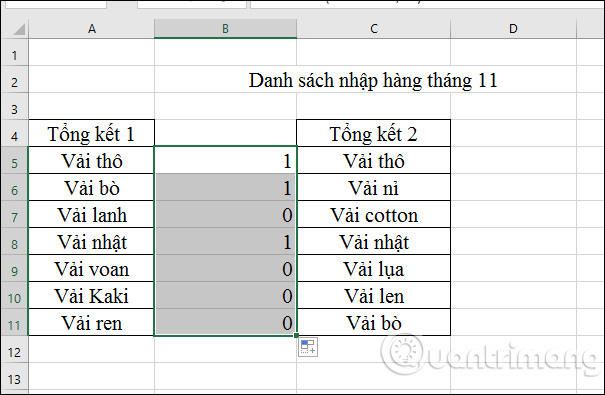
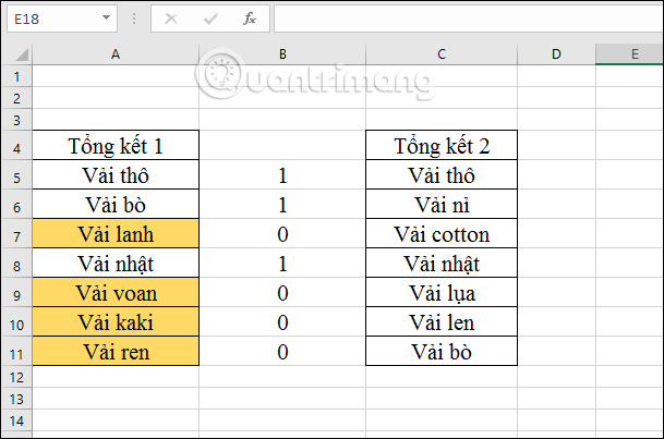
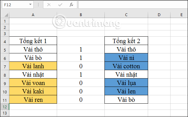
The result will be 1 as shown below. That means there will be 1 Raw Fabric data that matches the column 2.

How to compare data on 2 Excel columns Picture 5

Scroll down below we will get the complete result, with the comparison of the data in column 1 with column 2. The number 1 will be the same value, such as the Fabric in column 1 and column 2. The number 0 is The value does not match, only Lace fabric in column 1 is not available in column 2.

How to compare data on 2 Excel columns Picture 6

Step 5:

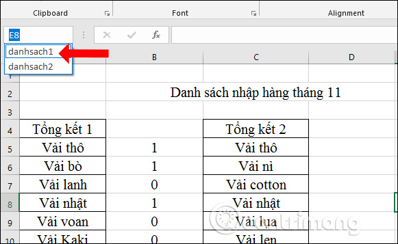
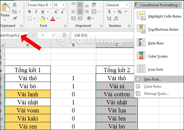
Next click on the Name box and then click on the triangle icon and select list1 .

How to compare data on 2 Excel columns Picture 7

Click on the Conditional Formatting item and then select New Rule. . in the drop down list.

How to compare data on 2 Excel columns Picture 8

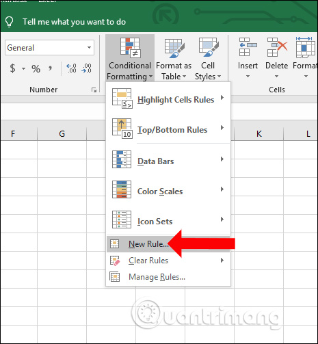
Step 6:

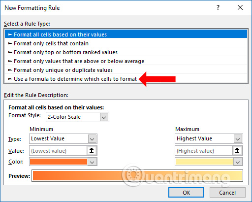
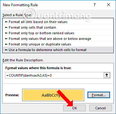
Display the new New Format Rule dialog box, click Use a formula to determine which cells to format .

How to compare data on 2 Excel columns Picture 9

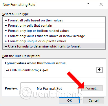
In the box below we enter the formula = COUNTIF (danhsach2, A5) = 0 . This means that you will find cells with a value of 0 in the list 1. Continue clicking the Format button .

How to compare data on 2 Excel columns Picture 10

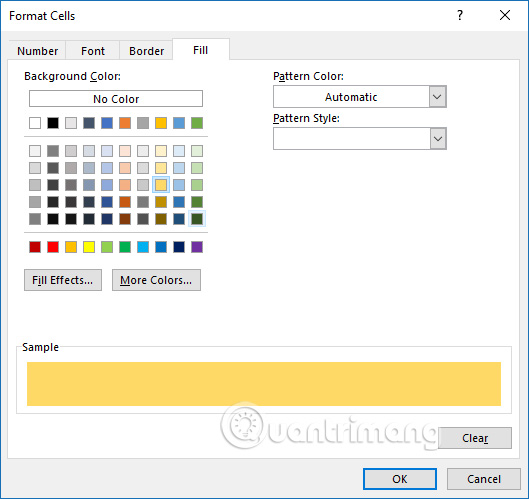
In the Format Cells dialog box, click the Fill tab and select the color to identify, click OK.

How to compare data on 2 Excel columns Picture 11

In the Preview section we will see the highlighted text you selected, click OK.

How to compare data on 2 Excel columns Picture 12

The results of the values ​​in column 1 not found in column 2 will be marked as shown.

How to compare data on 2 Excel columns Picture 13

Step 7:

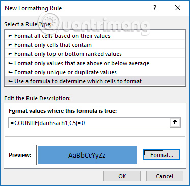
With the second list, users also click on the Name box to select list 2 . Then click on Conditional Formatting and select New Rule .

How to compare data on 2 Excel columns Picture 14

Next, enter the formula = COUNTIF (list1, C5) = 0 to find the value 0 in the second column.   Select the color and click OK.

How to compare data on 2 Excel columns Picture 15

The result will be as shown below. The different data on both tables will be colored to make it easier for statistics and inventory.

How to compare data on 2 Excel columns Picture 16

So with COUNTIF function in Excel we will know the number of data is the same when comparing between 2 columns. Data that does not match will be marked in the document.

See more:

1. 2 ways to separate column Full and Name in Excel
2. How to insert watermark, logo sink into Excel
3. Instructions for separating column content in Excel

I wish you all success!