How to Add Columns in a Pivot Table

Today's TipsMake will show you how to create and insert new columns into a pivot table on Microsoft Excel using the Pivot Table tool. You can change existing rows, fields, or data into columns, or create columns of calculated data using custom formulas.

Change data fields to columns

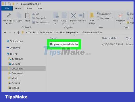
How to Add Columns in a Pivot Table Picture 1

Open the Excel file with the pivot table you want to edit. Find and double-click the Excel file on your computer to open it.

If you haven't created a pivot table yet, open a new Excel document and create a Pivot Table before continuing.

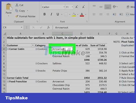
How to Add Columns in a Pivot Table Picture 2

Click any cell in the pivot table to select it. The Pivot Table Analyze and Design tabs appear in the tools ribbon at the top of the screen.

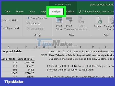
How to Add Columns in a Pivot Table Picture 3

Click the Pivot Table Analyze tab at the top. This tab is located alongside other tabs (such as Formulas, Insert, and View) at the top of the application window. The Pivot Table tool appears in the tools ribbon.

On some versions, this tab is called Analyze for short or appears as an option under the "Pivot Table Tools" heading.

How to Add Columns in a Pivot Table Picture 4

Click the Field List button in the ribbon. This button is to the right of the Pivot Table Analyze tab. A list of all fields, rows, columns, and values in the selected table will appear.

How to Add Columns in a Pivot Table Picture 5

Check the box next to any item in the FIELD NAME list. The sum of the original data in the category you select will be calculated and added to the pivot table as a new column.

Typically, non-numeric data fields are added as rows, while metric fields are added as columns by default.

You can uncheck the check box here at any time to delete the column.

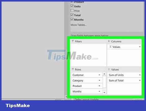
How to Add Columns in a Pivot Table Picture 6

Drag any field, row of data, or item of value and drop it into the "Columns" section. The selected category will automatically be moved to the Columns list and the pivot table will be redesigned with the newly added column.

Add calculated fields

How to Add Columns in a Pivot Table Picture 7

Open the Excel document you want to edit. Double-click the Excel document that contains your pivot table.

If you haven't created a pivot table yet, open a new Excel document and create a Pivot Table before continuing.

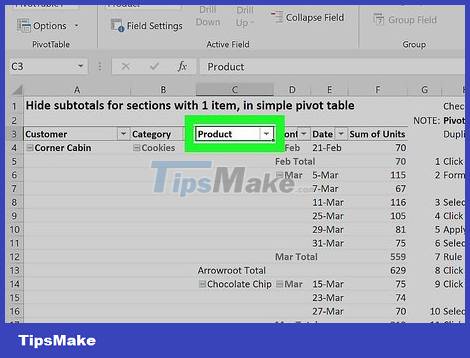
How to Add Columns in a Pivot Table Picture 8

Select the pivot table you want to edit. Click Pivot Table on the spreadsheet to select and edit.

How to Add Columns in a Pivot Table Picture 9

Click the Pivot Table Analyze tab . This tab is located in the middle of the tool ribbon at the top of the Excel window. The Pivot Table tool opens on the tools ribbon.

On some versions, this tab is called Analyze for short or appears as an option under the "Pivot Table Tools" heading.

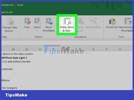
How to Add Columns in a Pivot Table Picture 10

Click the Fields, Items, & Sets button in the tools ribbon. This button has the word "fx" in the table icon at the bottom right of the toolbar. A drop-down menu will appear.

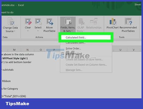
How to Add Columns in a Pivot Table Picture 11

Click Calculated Field in the drop-down menu. A window for you to add a new custom column to the Pivot Table will open.

How to Add Columns in a Pivot Table Picture 12

Enter a name for the column in the "Name" field. Click the Name data field and enter the name you want for the new column. This name will appear at the top of the column.

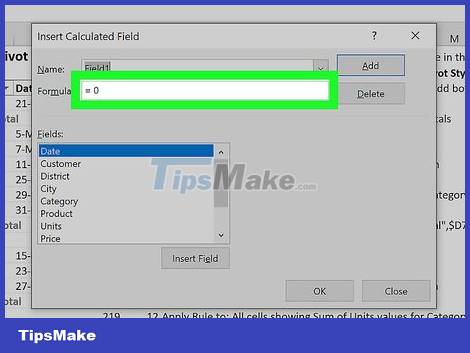
How to Add Columns in a Pivot Table Picture 13

Enter the formula for the new column in the "Formula" field. Click the Formula data field below the Name field and enter the formula you want to use to calculate the data value in the new column.

You need to make sure you enter the formula to the right of the "=" sign.

Or you can also select an existing column and add it to the formula as a value. Select the field you want to add to the data fields section here and click Insert Field to insert it into the formula.

How to Add Columns in a Pivot Table Picture 14