Excel 2019 (Part 6): Formatting Cells

In Microsoft Excel , all cell contents use the same formatting by default, which can make reading a workbook with a lot of information difficult. Basic formatting allows you to customize the look and feel of your workbook, letting you draw attention to specific sections and making the content easier to view and understand.

 

How to change the font size

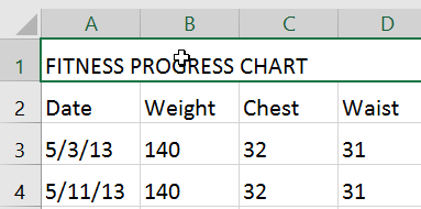
1. Select the cell(s) you want to modify.

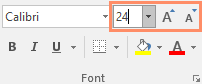
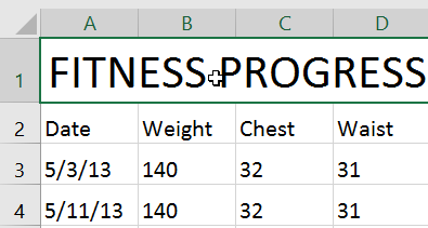
2. On the Home tab , click the drop-down arrow next to the Font Size command , then select your desired font size. For example, you would choose size 24 to make the text larger.

 

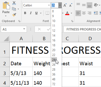
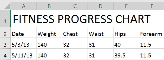
3. The text will change to the selected font size.

You can also use the Increase Font Size and Decrease Font Size commands , or enter a custom font size using the keyboard.

 

How to change the font

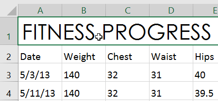
By default, the font of each new workbook is set to Calibri. However, Excel offers many other fonts that you can use to customize the text in your cells. The example below will format the header cell to help distinguish it from the rest of the worksheet.

1. Select the cell(s) you want to modify.

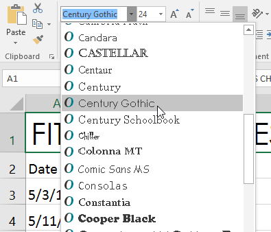
2. On the Home tab , click the drop-down arrow next to the Font command , then select your desired font. For example, we would choose Century Gothic.

 

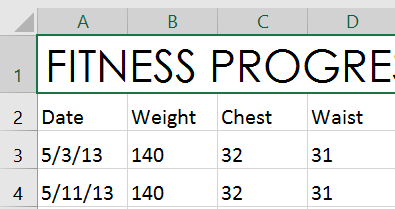
3. The text will change to the selected font.

When creating workbooks at work, you'll want to choose a font that's easy to read. Along with Calibri, standard readable fonts include Cambria, Times New Roman, and Arial.

How to change the font color

1. Select the cell(s) you want to modify.

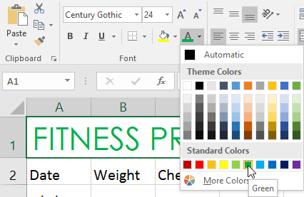
2. On the Home tab , click the drop-down arrow next to the Font command , then select your desired font color. For example, we will choose green.

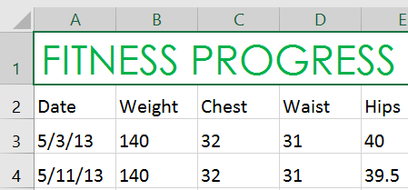
3. The text will change to the selected font color.

 

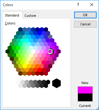
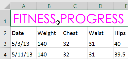
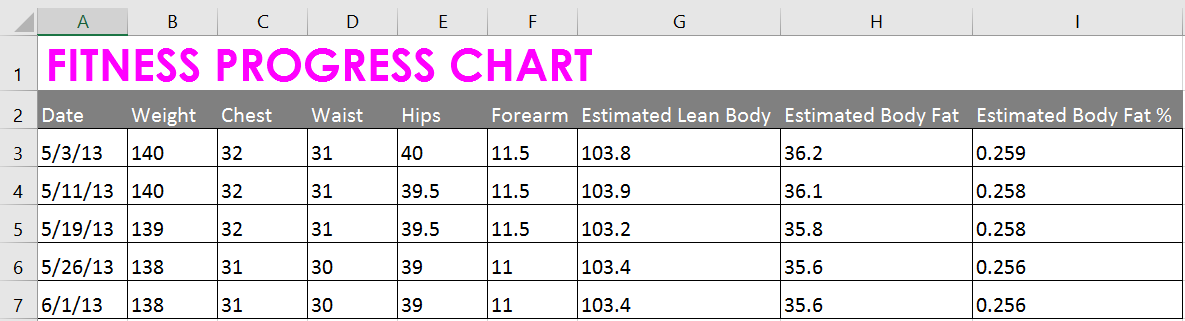
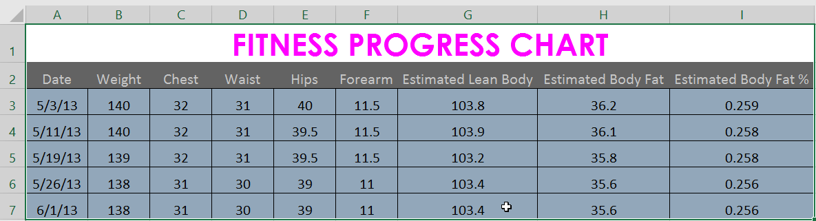
Select More Colors at the bottom of the menu to access additional color options. The example has changed the font color to bright pink.

Use the bold, italic, and underline commands.

1. Select the cell(s) you want to modify.

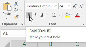
2. Click the bold ( B ), italic ( I ), or underline ( U ) command on the Home tab. The example will bold the selected cells.

3. The selected style will be applied to the text.

 

You can also press Ctrl + B on your keyboard to bold the selected text, Ctrl + I to apply italics, and Ctrl + U to apply an underscore.

Cell border and background color

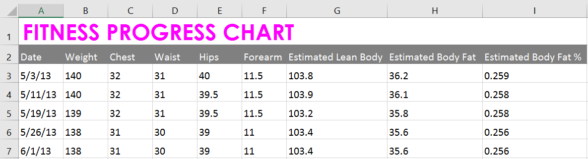
Cell borders and background colors allow you to create clear and defined boundaries for different sections of a worksheet. Below, the example will add cell borders and background colors to header cells to help distinguish them from the rest of the worksheet.

How to add a background color

1. Select the cell(s) you want to modify.

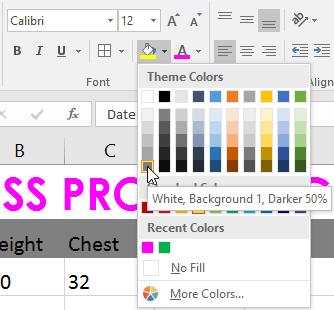
2. On the Home tab , click the drop-down arrow next to the Fill Color command , then select the background color you want to use. For example, we will choose dark gray.

3. The selected background color will appear in the selected cells. The example also changed the font color to white to make it easier to read with this new background color.

How to add a border

1. Select the cell(s) you want to modify.

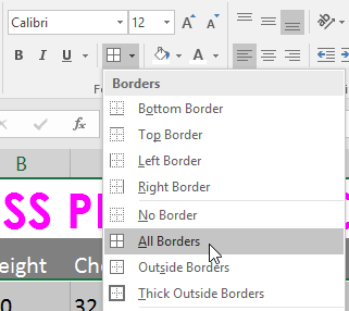
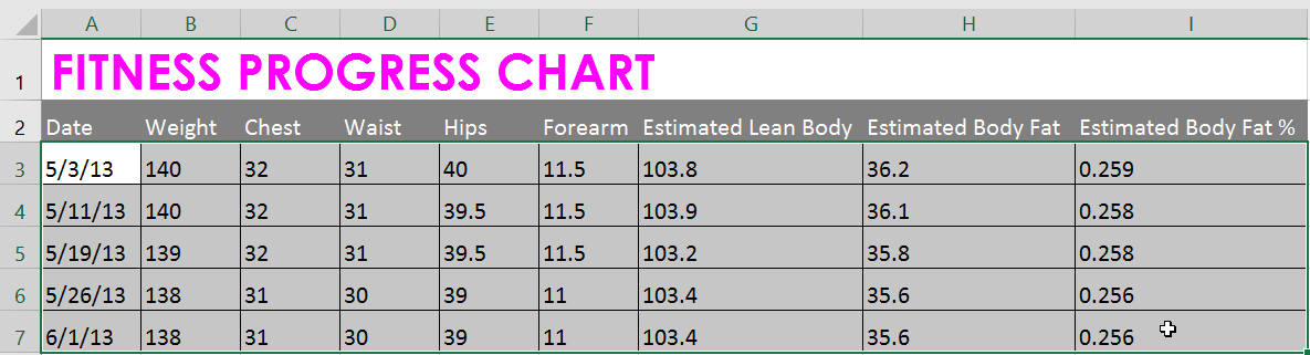
2. On the Home tab , click the drop-down arrow next to the Borders command , then select the border style you want to use. For example, we will select to display All Borders.

 

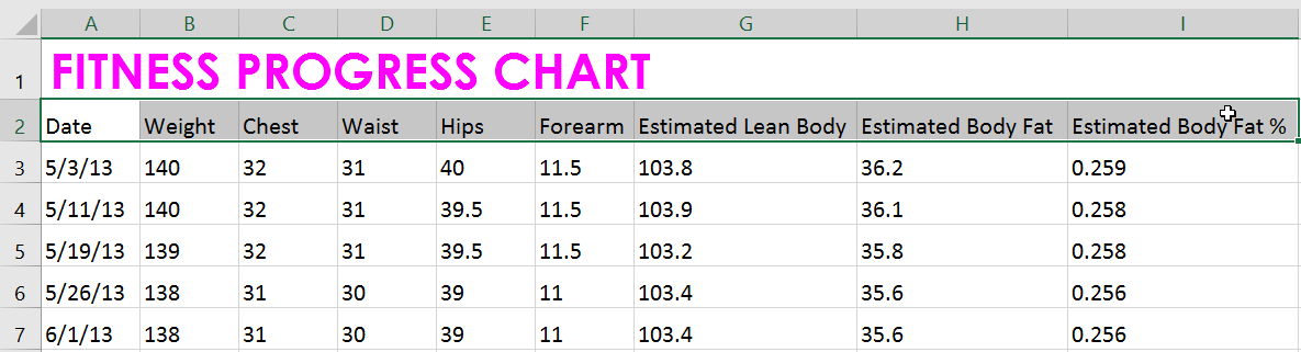
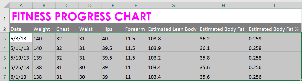
3. The selected border style will appear.

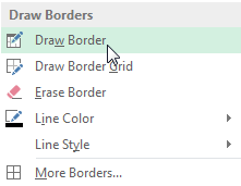
You can draw borders and change their style and color using the Draw Borders tool at the bottom of the Borders drop-down menu .

Cell type

Instead of manually formatting cells, you can use Excel's pre-designed styles. Cell styles are a quick way to include professional formatting for different parts of a workbook, such as the title and header.

How to apply cell type

This example will apply a new cell style to the existing title and header cells.

1. Select the cell(s) you want to modify.

2. Click the Cell Styles command on the Home tab , then select your desired style from the drop-down menu.

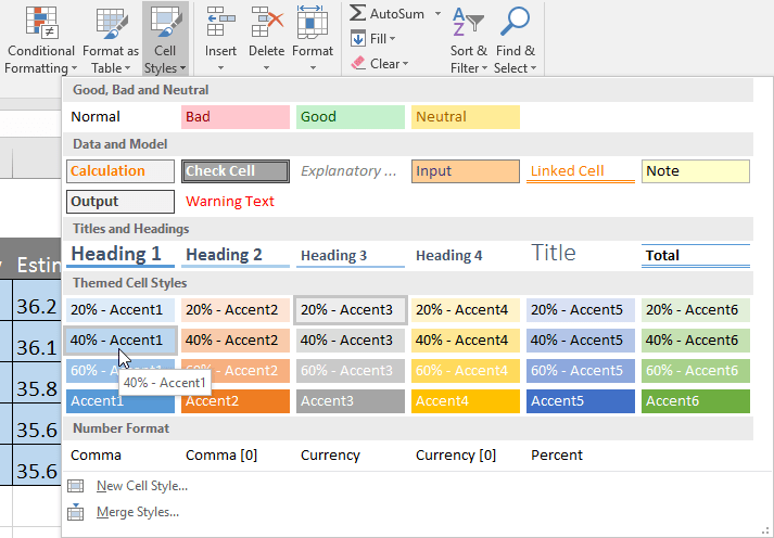
3. The selected cell type will appear.

Applying cell styles will override all existing formatting except for text alignment. You may not want to use cell styles if you have already added a lot of formatting to your workbook.

Text alignment

By default, any text entered into a spreadsheet will be aligned to the bottom left of the cell, while numbers will be aligned to the bottom right. Changing the cell alignment allows you to choose how content is displayed in any cell, which can make your content easier to read.

1. Left Align : Align the content to the left border of the cell.
2. Center Align : Aligns the content equally from the left and right borders of the cell.
3. Right Align : Align the content to the right border of the cell.
4. Top Align : Align the content to the top border of the cell.
5. Middle Align : Aligns the content equally from the top and bottom borders of the cell.
6. Bottom Align : Align the content to the bottom border of the cell.

How to change the horizontal text alignment

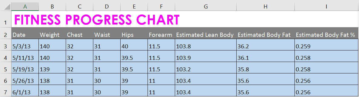
The example below will modify the alignment of the header cell to better distinguish it from the rest of the worksheet.

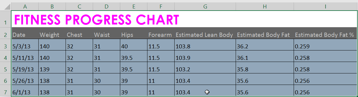
1. Select the cell(s) you want to modify.

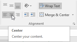
2. Select one of the three horizontal alignment commands on the Home tab. For example, we would select Center Align .

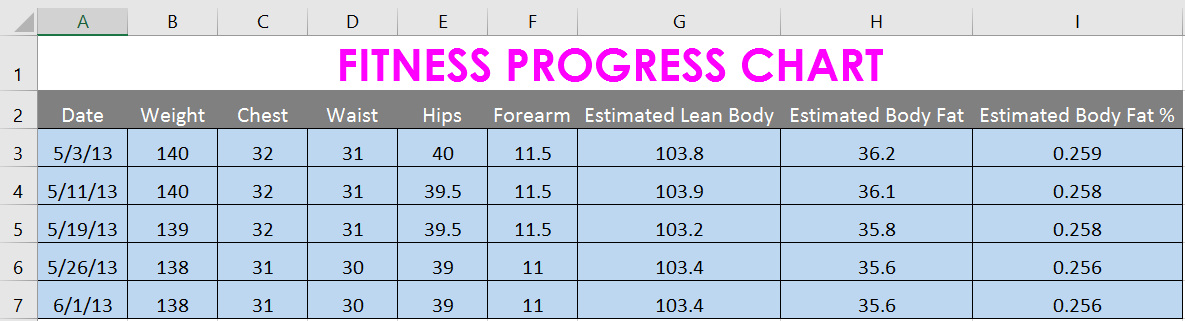
3. The text will be redesigned.

How to change the vertical alignment of text

1. Select the cell(s) you want to modify.

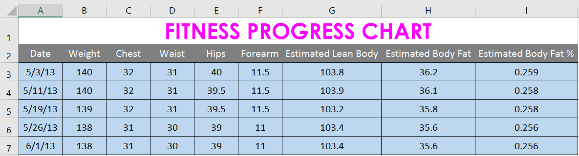
2. Select one of the three vertical alignment commands on the Home tab. For example, we would select Middle Align.

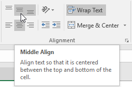
3. The text will be readjusted.

You can apply both vertical and horizontal alignment settings to any cell.

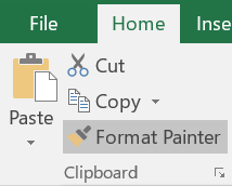
Format Painter

If you want to copy formatting from one cell to another, you can use the Format Painter command on the Home tab. When you click Format Painter , it will copy all the formatting from the selected cell. Then, you can click and drag it to any cell where you want to paste the formatting.