Excel 2019 (Part 5): Modifying Columns, Rows, and Cells

By default, all rows and columns in a new workbook are set to the same height and width. Microsoft Excel allows you to modify column widths and row heights in various ways, including applying the Text Wrapping feature and merging cells .

 

How to modify column width

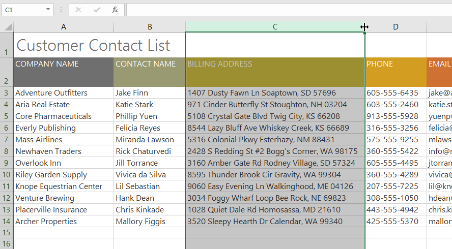
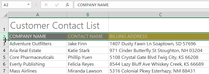
In the example below, column C is too narrow to display all the content in these cells. It's possible to display all of this content by changing the width of column C.

1. Place your mouse cursor over the column row in the column header so that the cursor changes to a double arrow.

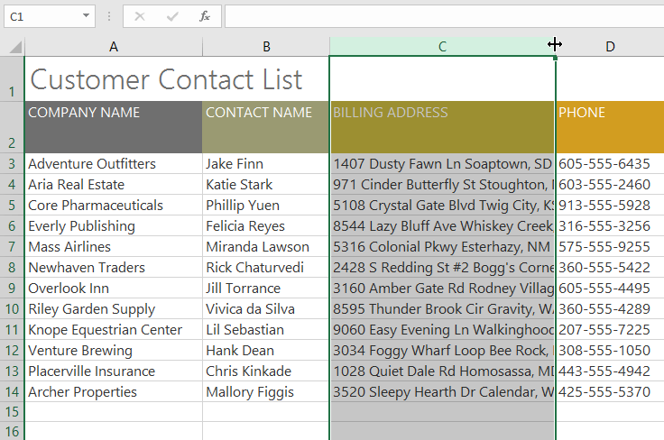
2. Click and drag the mouse to increase or decrease the column width.

 

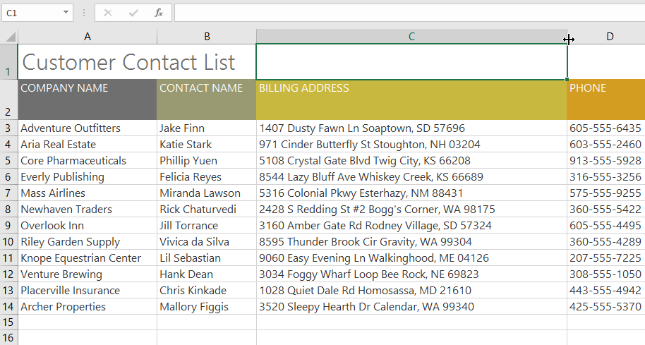
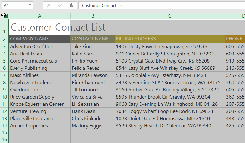
3. Release the mouse button. The column width will change.

With numerical data, the cell will display a hash symbol (#######) if the column is too narrow. Simply increase the column width to display the data.

AutoFit feature

The AutoFit feature will allow you to set the column width to automatically fit its content.

1. Place your mouse cursor over the column row in the column header so that the cursor changes to a double arrow.

2. Double-click. The column width will automatically adjust to fit the content.

 

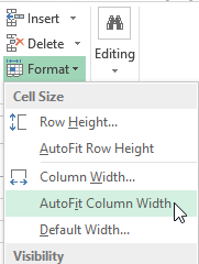
You can also apply AutoFit to the width of several columns at once. Simply select the columns you want to apply AutoFit to, then select the AutoFit Column Width command from the Format drop-down menu on the Home tab. This method can also be used for row height.

How to modify row height

1. Place the cursor on the line so that the cursor becomes a double arrow.

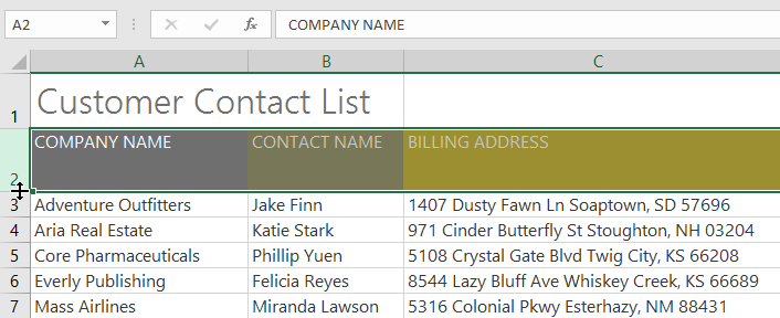
2. Click and drag the mouse to increase or decrease the height of the row.

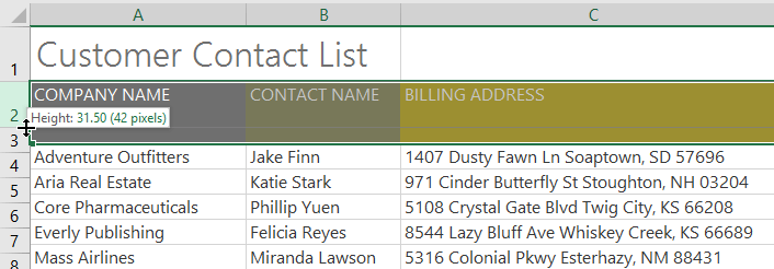
3. Release the mouse button. The height of the selected row will be changed.

How to modify all rows or columns

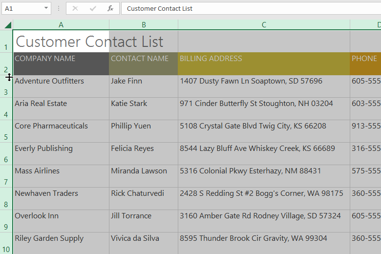
Instead of resizing individual rows and columns, you can modify the height and width of every row and column at once. This method allows you to set a uniform size for all rows and columns in your spreadsheet. The example will set a uniform row height.

1. Locate and click the Select All button just below the name box to select all cells in the worksheet.

 

2. Place your mouse cursor over a line so that the cursor becomes a double arrow.

3. Click and drag the mouse to increase or decrease the row height, then release the mouse when you are satisfied. The row height will be changed for the entire worksheet.

Insert, delete, move, and hide.

After working with workbooks for a while, you might find that you want to insert new columns or rows, delete certain rows or columns, move them to a different location in the worksheet, or even hide them.

How to insert rows

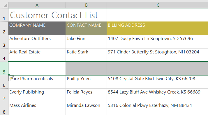
1. Select the row header below where you want the new row to appear. For example, if you want to insert a row between rows 4 and 5, then row 5 will be selected.

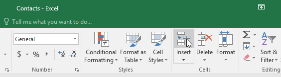
2. Click the Insert command on the Home tab.

3. A new row will appear above the selected row.

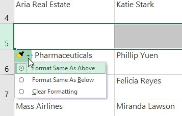
When inserting new rows, columns, or cells, you'll see a paintbrush icon next to the inserted cells. This button lets you choose how Excel formats these cells. By default, Excel formats inserted rows to have the same formatting as the cells in the row above. To access additional options, hover over the icon, then click the drop-down arrow.

How to insert columns

 

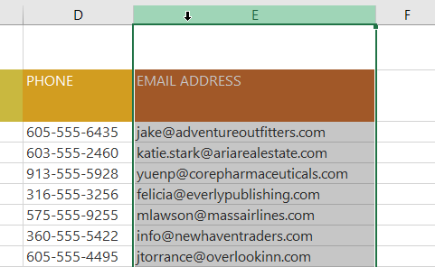
1. Select the column header to the right of where you want the new column to appear. For example, if you want to insert a column between columns D and E, select column E.

2. Click the Insert command on the Home tab.

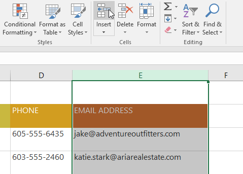
3. A new column will appear to the left of the selected column.

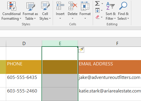
When inserting rows and columns, make sure to select the entire row or column by clicking on the header. If you only select a cell in the row or column, the Insert command will only insert a new cell.

How to delete a row or column

It's easy to delete a row or column that you no longer need. For example, deleting a row would delete a column, but you can delete a column in the same way.

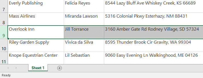
1. Select the row you want to delete. For example, we would select row 9.

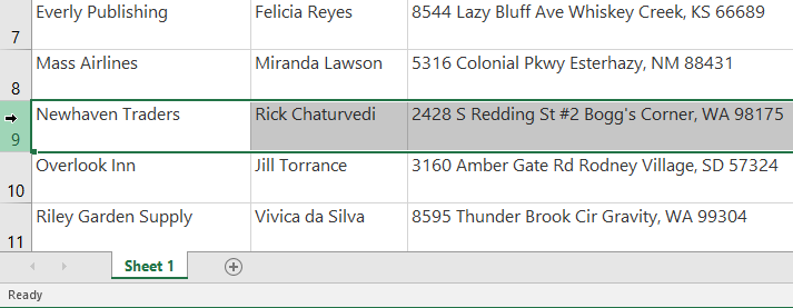
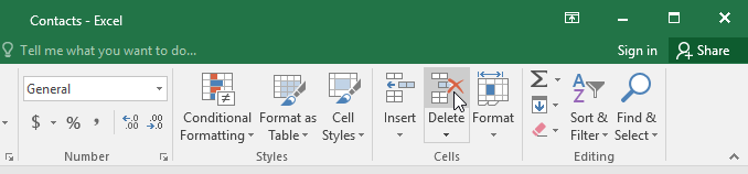
2. Click the Delete command on the Home tab.

3. The selected row will be deleted and the surrounding rows will change. In the example, row 10 has been moved up, so it is now row 9.

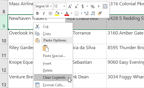
It's important to understand the difference between deleting a row or column and deleting its contents. If you want to delete the contents of a row or column without affecting other rows and columns, right-click a header, then select Clear Contents from the drop-down menu.

How to move a row or column

Sometimes you might want to move a column or row to rearrange the contents of your spreadsheet. For example, this would move a column, but you can move a row in a similar way.

1. Select a header for the column you want to move.

 

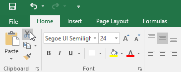
2. Click the Cut command on the Home tab or press Ctrl + X on your keyboard.

3. Select the column header to the right of where you want to move the column. For example, if you want to move a column between columns E and F, select column F.

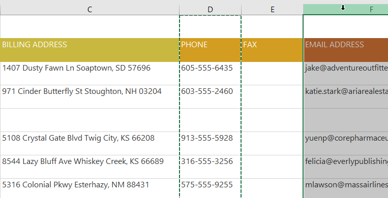
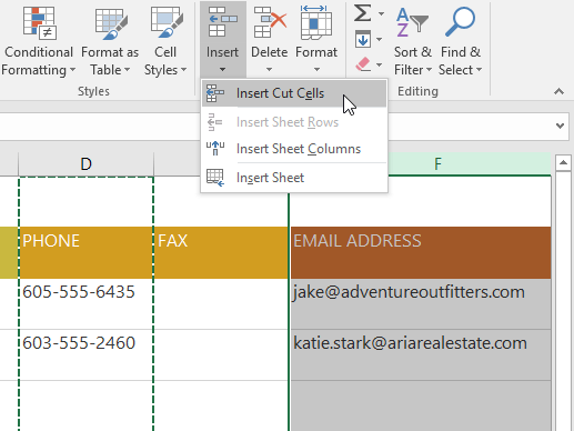
4. Click the Insert command on the Home tab , then select Insert Cut Cells from the drop-down menu.

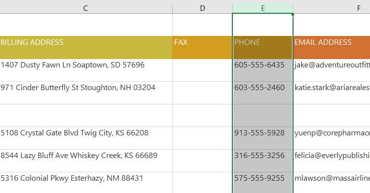
5. The column will be moved to the selected position, and the surrounding columns will shift.

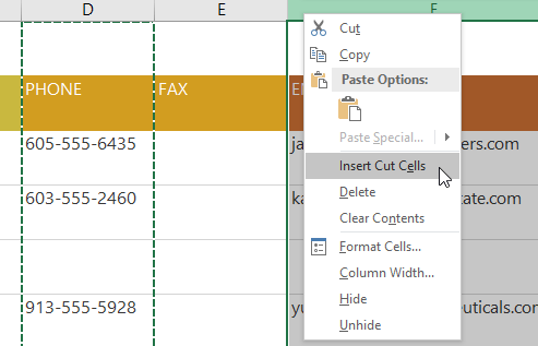
You can also access the Cut and Insert commands by right-clicking and selecting the desired commands from the drop-down menu.

How to hide/show a row or column

Sometimes, you might want to compare certain rows or columns without changing the spreadsheet's organization. To do this, Excel allows you to hide rows and columns as needed. The example will hide a few columns, but you can hide rows in a similar way.

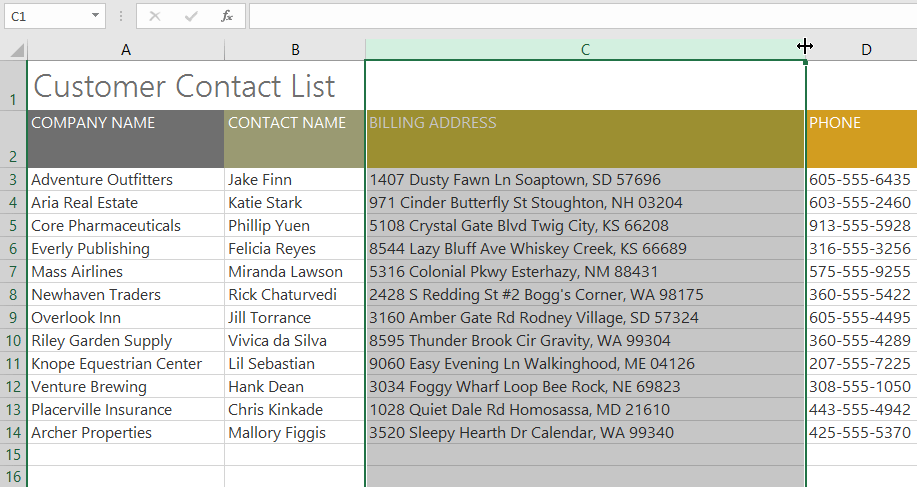
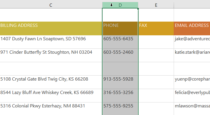
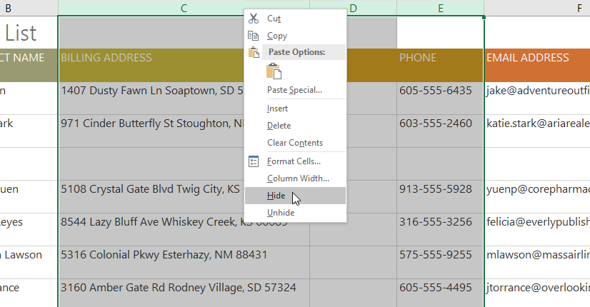
1. Select the columns you want to hide, right-click, and then select Hide from the Format menu. For example, this will hide columns C, D, and E.

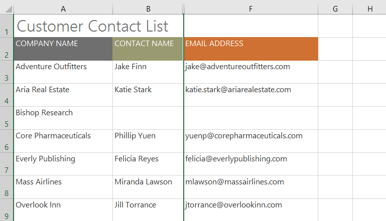
2. The columns will be hidden. The green column line indicates the location of the hidden columns.

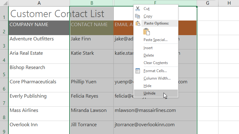
3. To show the columns, select the columns on both sides of the hidden column. For example, we would select columns B and F. Then, right-click and select Unhide from the formatting menu.

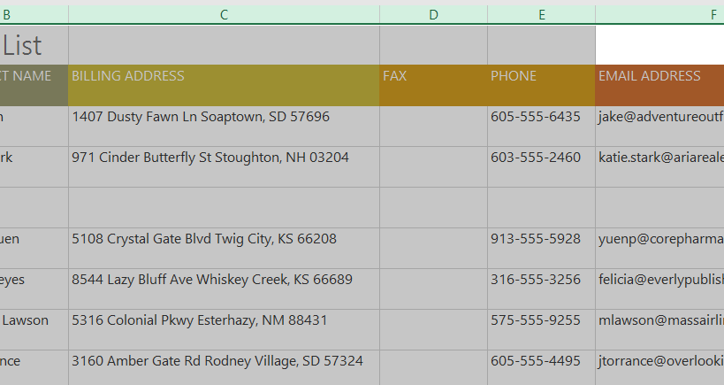
4. The hidden columns will reappear.

Text Wrap and merge cells

 

Whenever you have too much content to display in a single cell, you can use the Text Wrap or merge cells feature instead of resizing the column. Text Wrap automatically modifies the cell's row height, allowing the cell's content to be displayed across multiple lines. Merge allows you to combine a cell with adjacent empty cells to create one large cell.

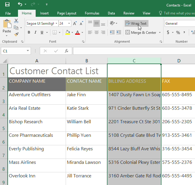
How to apply Text Wrap in cells

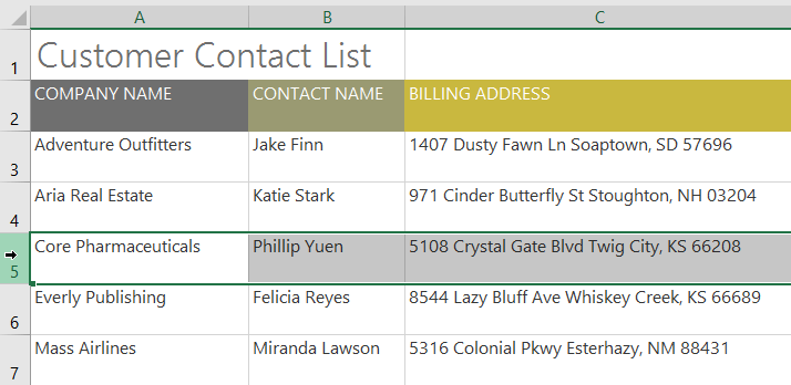
1. Select the cells you want. For example, we will select the cells in column C.

2. Click the Wrap Text command on the Home tab.

3. The text in the selected cells will be merged.

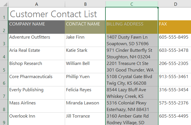
Click the Wrap Text command again to return the text to its original state.

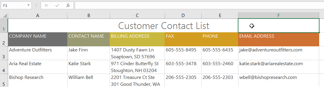
How to merge cells using the Merge & Center command.

1. Select the range of cells you want to merge. For example, we would select A1:F1.

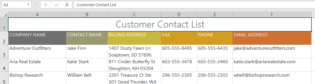
2. Click on the Merge & Center command on the Home tab.

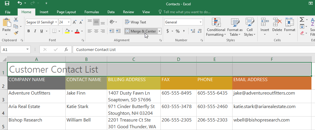
3. The selected cells will be merged and the text will be centered.

How to access additional merge options

If you click the drop-down arrow next to the Merge & Center command on the Home tab, the Merge drop-down menu will appear.

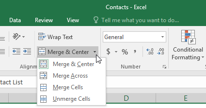
From here, you can choose:

1. Merge & Center : This action merges the selected cells into one and centers the text.
2. Merge Across : This option merges the selected cells into larger cells while keeping each row separate.
3. Merge Cells : This option merges the selected cells into one, but does not center the text.
4. Unmerge Cells : This operation cancels the merging of the selected cells.

Be careful when using this feature. If you merge multiple cells that all contain data, Excel will only keep the contents of the top-left cell and discard everything else.

Center Across Selection feature

Merging cells can be helpful for organizing your data, but it can also create problems later on. For example, it can be difficult to move, copy, and paste content from merged cells. A good alternative to merging is the Center Across Selection feature, which creates a similar effect without actually merging cells.

How to use Center Across Selection

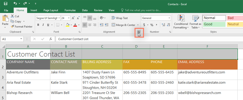
1. Select the desired range of cells. For example, we would select A1:F1. Note: If you have merged these cells, you should unmerge them before proceeding to step 2.

2. Click the small arrow in the lower right corner of the Alignment group on the Home tab.

3. A dialog box will appear. Locate and select the Horizontal drop-down menu , choose Center Across Selection , and then click OK.

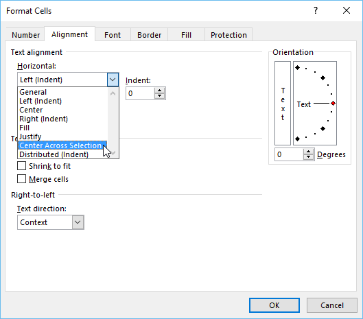
4. The content will be centered within the selected cell range. As you can see, this produces a visual result similar to the merge and center option, but preserves each cell within A1:F1.