How to Create a Filter in an Excel Cell

This guide explains how to create a Filter in an Excel Cell, with clear steps, practical tips, and important checks before you begin.

Today, Dexterity Software will guide readers in the most detailed way how to create filters in an Excel cell.

Consider the specific example as follows, need to create a list of products including: Men's shirts, Women's shirts, Women's dresses so the importer selects a product item from the list you have created.

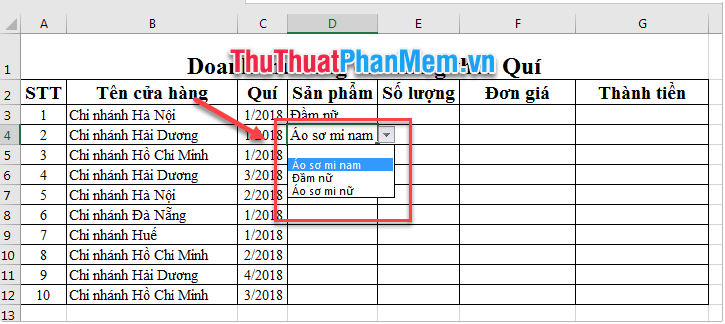
The way to do this is as follows:

Step 1: Create a product listing on a separate worksheet.

Create a new sheet, enter the product entries you want included in your drop-down list.

Step 2: Convert the product list to a table ( Table ) in Excel.

• Select any cell in the data area containing the product list. Press the key combination Ctrl + T .
• Create Table window appears, if your data contains headlines, click My table has headers , if not, then uncheck.
• Click the OK button to set the Table table.

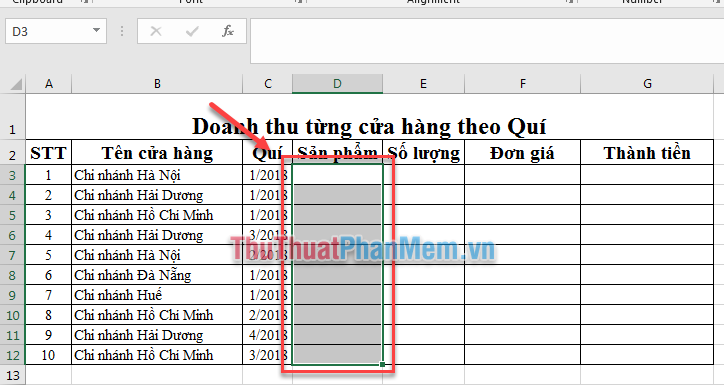
Step 3: Return to the working worksheet. Select the cells in the worksheet you want to place the drop-down list.

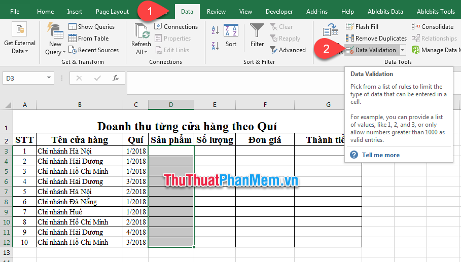
Step 4: On the Data tab (1) => Click on the Data Validation icon (2) .

Step 5: Data Validation window appears. On the Settings tab , Allow (1), click List .

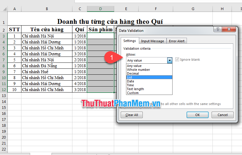
The Source (2) section selects the range of item ranges your product created in Step 1 .

Note that you omit the subject line because otherwise, the subject line will form another option.

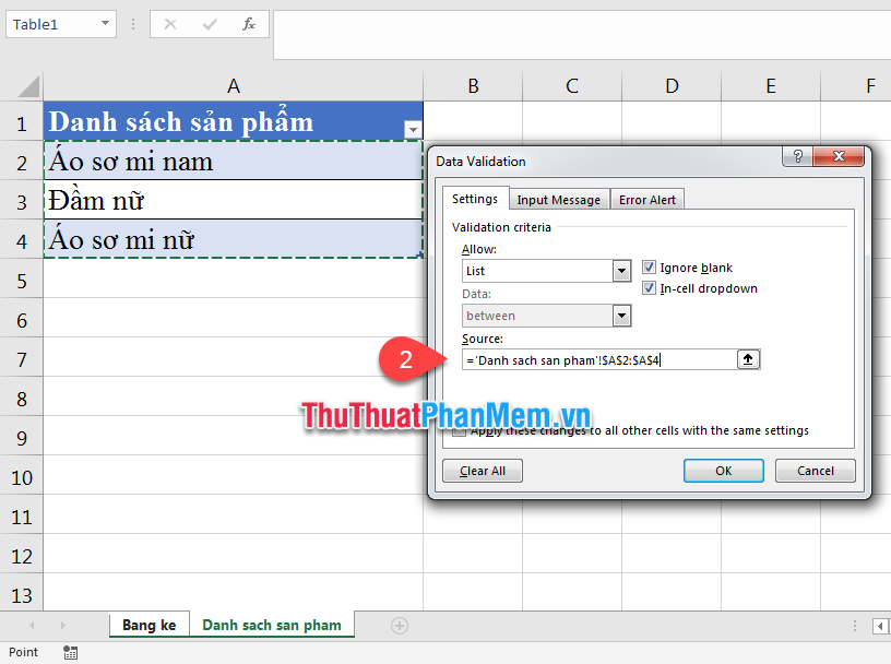
• If you want the user to leave the box blank, select Ignore blank , if you force users not to leave the box blank, uncheck the box.
• Select In-cell dropdown (filter box to select options).

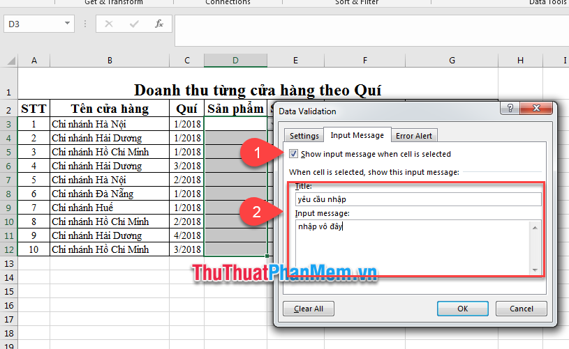
Step 6: Switch to the Inut messeger tab.

If you want a notification to pop up when the user clicks on that box, select the Show input messeger when cell is selected (1) check box , then type the title and content you want to notify (2) (maximum 225 characters). If you do not want to be shown, deselect this item.

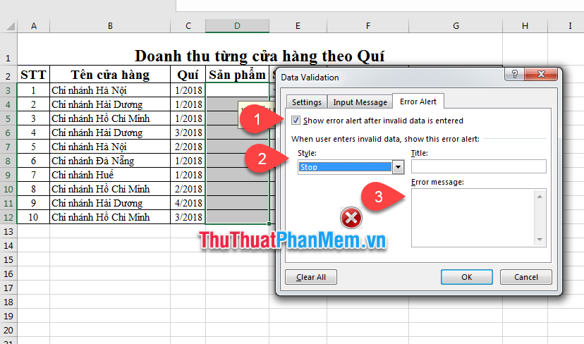
Step 7: The Error Alert tab is used to set up an error warning if the person who entered the product item is not in the list you created at the beginning.

If you want Excel software to report errors, select the Show error alert after invalid data is entered (1) check box .

Select the symbols that appear in the case of errors in Style (2) and enter the title and message content (3) if necessary.

Step 8: Click the OK button to start running Data Validation . The result is:

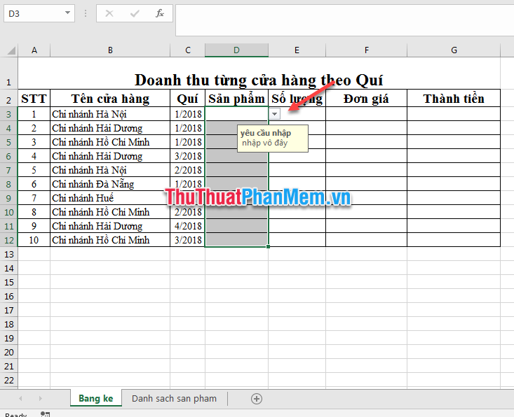
When you click on a cell where you have Validation installed, the selection arrow box will appear to the right of the cell, click the arrow and select items from the previously created list.

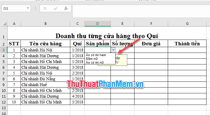
Or you can type the item directly into the cell. If you make a mistake, Excel will display a warning window:

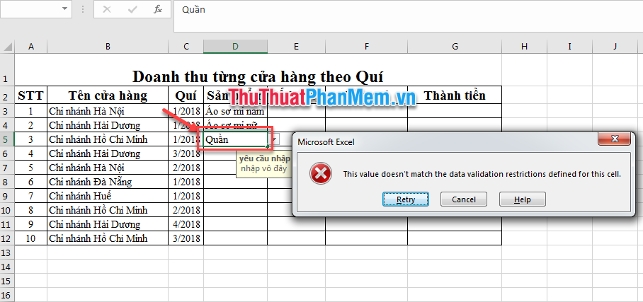
In this case you just need to press the Entry button and re-enter the correct data.

Above Software Tips guide you how to create drop down lists with tools available in Excel. Good luck!