100 extremely useful Excel tips to know - Part 2

In this article, we present 100 more useful Excel tips that you need to know Part 2 to help you adjust the speed and get the most out of it.

22. Set password to protect Excel file

You need to secure the data on Excel files, only the person who is provided with the password can see the content details. The easiest way is to create a password for Excel file by going to Review -> Protect Workbook:

100 extremely useful Excel tips to know - Part 2 Picture 1

Enter the password to protect the file, so before opening the Excel file ask you for the password if the password is correct so you can see the contents of the file.

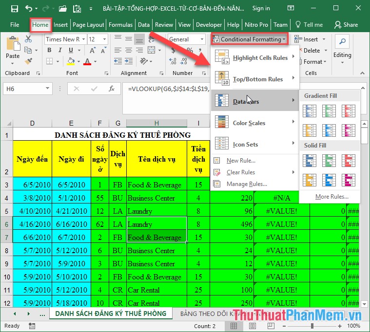
23. Magician in Excel with Conditional Formating

Regrettably, if you omit this feature, it is an extremely useful feature that helps you conditionally format many attributes of the object, such as coloring the values ​​to satisfy conditions, attention .

100 extremely useful Excel tips to know - Part 2 Picture 2

24. Join your name, creating a space in the middle

You have data columns that contain last names, middle names, the name you want to combine them into a single data column full of fields, middle names, first name. Very simple you just need to use & & insert space characters between words.

100 extremely useful Excel tips to know - Part 2 Picture 3

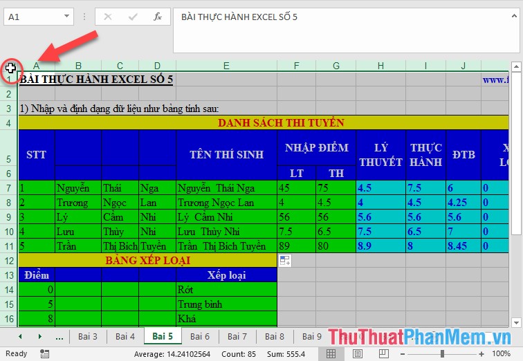
25. Select all data with 1 mouse click

To select all the data, you just need to click on the first cell on the top left of the worksheet, which is extremely useful when you need to format the worksheet:

100 extremely useful Excel tips to know - Part 2 Picture 4

26. Hide cell data

In order for users to not be able to see the data of the cell, but the data is still displayed in the formula bar to serve the calculation you just select the data area you want to hide -> right-click and select Format Cell -> select Custom -> enter 3 semicolons in Type:

100 extremely useful Excel tips to know - Part 2 Picture 5

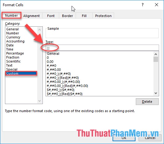
The data results are hidden, especially in this way you apply to data types:

100 extremely useful Excel tips to know - Part 2 Picture 6

27. How to capitalize, print faster

You have accidentally entered data in uppercase (or lowercase) but according to the standard you must enter lowercase (uppercase), do not rush to delete and re-enter, you use the function available in Excel:

- To convert uppercase to lowercase, use the Lower () function

- To convert lowercase to uppercase using the UpCase () function

For example:

100 extremely useful Excel tips to know - Part 2 Picture 7

28. Open multiple Excel files at once

Your folder contains many Excel files and you want to open all those files, instead of clicking each file individually -> press Ctrl + A to select all those files -> press Enter as So you can open many Excel files at the same time with only one operation.

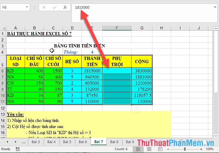
29. Convert data thousands and millions into k and m

215k is the current common abbreviation, which helps to shorten numerical values, and helps to calculate faster. This is not difficult, you just need to select the data area you want to convert units k, m-> right-click select Format Cell or press Ctrl + 1 -> the dialog box appears select Custom -> type Input '# ## ',' k '-> click OK:

100 extremely useful Excel tips to know - Part 2 Picture 8

The result you created the data with unit k:

100 extremely useful Excel tips to know - Part 2 Picture 9

Similar to the type m, you operate as above.

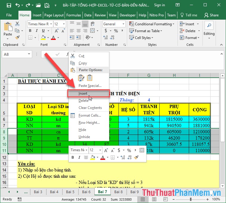
30. Add multiple lines at once in Excel

To add multiple lines at once, select the number of rows to add -> right-click and choose Insert, you will add the number of rows exactly equal to the number of rows you have scanned, for example:

100 extremely useful Excel tips to know - Part 2 Picture 10

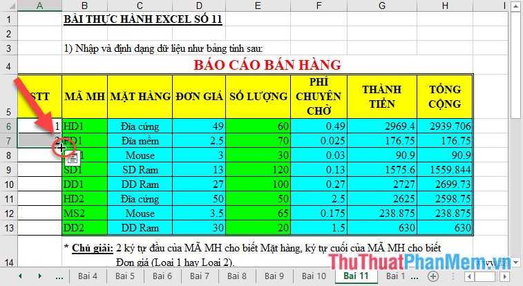
31. Automatically fill 1 series

Numbering is not really difficult, but when the list reaches thousands of records, using the drag and drop is not reasonable and very difficult. To fill in the column no, follow these steps:

Step 1: Enter the full content in addition to STT

Step 2: Enter the first 2 values ​​of the STT column -> select the 2 cells entered -> appear the black plus sign -> double click on the icon -> you have filled stt to the last row containing data Whether. Note the lines must be contiguous, no spaces, no blank lines:

100 extremely useful Excel tips to know - Part 2 Picture 11

32. Quickly format tables in Excel

Instead of manipulating multiple times, simply press the key combination Alt + H + T dialog box appears select the type to format:

33. Freeze the first column and column

To freeze rows, the first column you go to View -> Freeze Panes tab includes the following options:

- Freeze Top Row: Freeze the first line

- Freeze First Column: Freeze the first column

100 extremely useful Excel tips to know - Part 2 Picture 12

34. Choose a random number on the spreadsheet

In case you want to generate random numbers, you don't need to think about using the Randbetween function (Bottom, Top) to help you generate random numbers, where Bottom and Top are limited to the range of random numbers. course created within that limit.

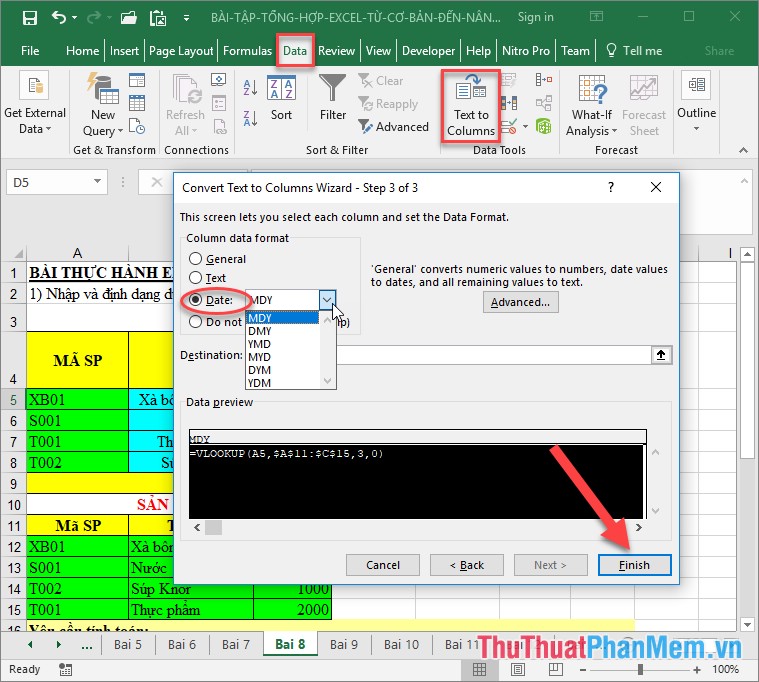
35. Convert numeric data to a date

To convert numeric data to date format, do the following: Select the data cell to be converted to Data tab -> Text to Column -> dialog box appears, click Next and continue to select the data type format Date -> Finish:

100 extremely useful Excel tips to know - Part 2 Picture 13

36. Filter data in Excel

Save a lot of time and effort when you select the data filtering feature in Excel. Just select the headline on the Data tab and select Filter:

100 extremely useful Excel tips to know - Part 2 Picture 14

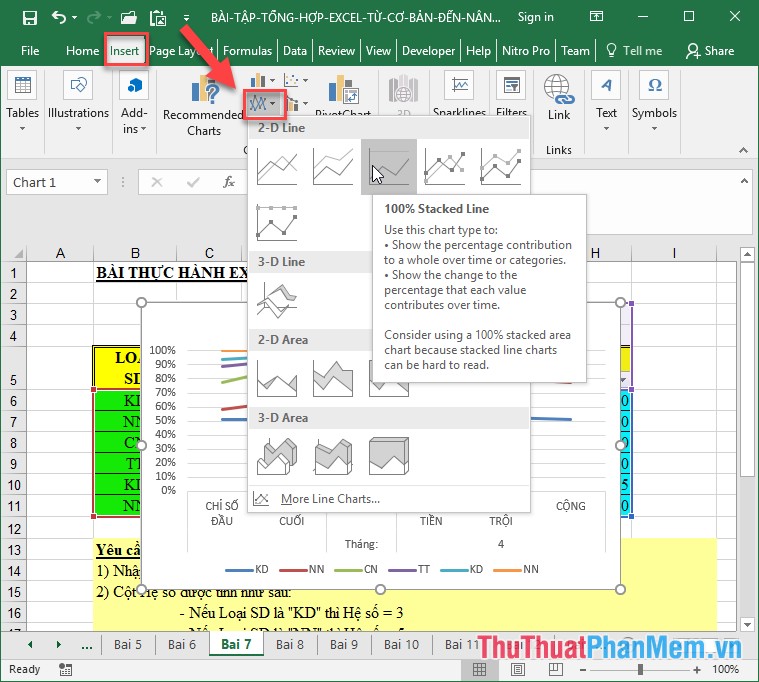
37. Use Sparkline in the chart

To make the diagram easier to understand, you need to insert Sparkline in the chart, very simple on the Insert tab -> Insert line or Area chart :

100 extremely useful Excel tips to know - Part 2 Picture 15

38. Change the default font after Excel

To change the default font, press Alt + T + F.

39. Interaction between English and Excel

An important issue you need to know when learning Excel is English, Fluent English is an advantage that helps you do a lot better than Excel.

40. Excel is an indispensable daily tool

Another simple way to help you learn Excel a lot better is to work regularly with Excel, without interruption, to help you always remember and do your job well.

41. Select data in an Excel cell

To quickly move in 1 cell you need to know the following shortcut:

- Shift + arrow keys left and right: move left, right 1 character.

- Ctrl + Shift + Arrow keys left and right: move left, right 1 word

- Shift + Home : Move to the beginning of the cell

- Shift + End : Move to the end position of the cell

42. Delete data in an Excel cell

- Delete data to the left of the mouse cursor and press the BackSpace key

- Delete data to the right of the mouse cursor and press the Delete key

- Delete data from the cursor position to the last position of the cell press Ctrl + Delete key combination

43. 'Enter' - enter data

A number of keyboard shortcuts with the Enter key assist you to type quickly:

- Enter: Go to the bottom of the line.

- Shift + Enter: Move up.

- Shift + tab: Move the cursor to the left.

- Tab: Move to the right

- Ctrl + Enter: Stand at the position of the mouse cursor.

44. Enter data for a data range

To enter data for a region, you only need to scan the data area -> enter content -> press Ctrl + Enter to move the input location, make sure you only enter data in the selected area.

45. Copy the formula from the cell to the bottom

To minimize mouse operations, you can use the following key combination when copying data:

- Press the key combination Ctrl + apostrophe : to copy the formula in the upper cell.

- Press the key combination Ctrl + Shift + apostrophe : to copy the formula in the box below.

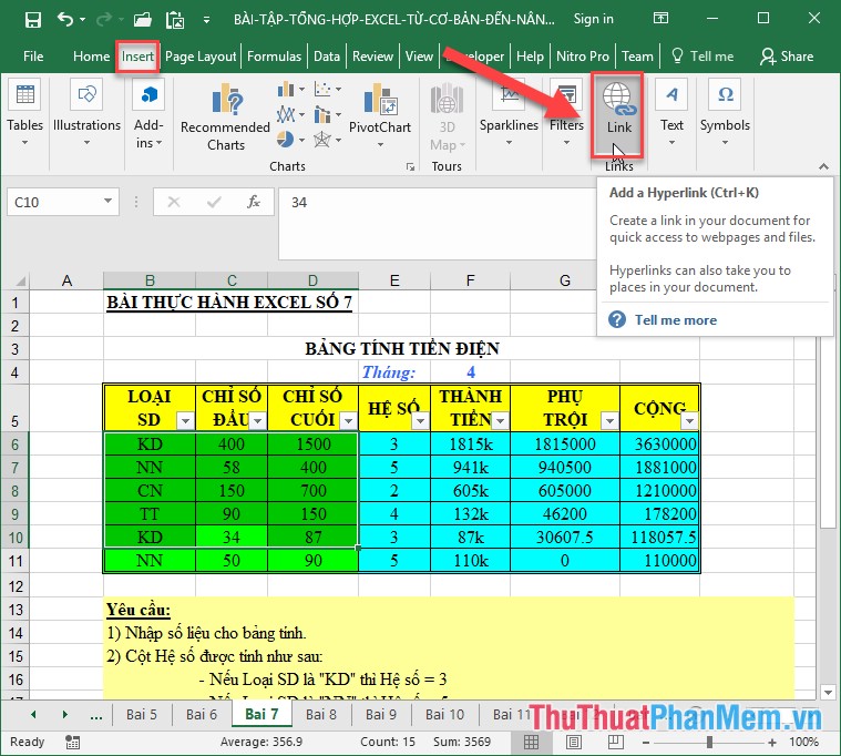
46. ​​Insert Hyperlink

To insert a link, click Insert  -> links:

100 extremely useful Excel tips to know - Part 2 Picture 16

47. Open the font settings dialog

Quick action when you select the font for the worksheet, you just need to press Ctrl + Shift + F.

48. Dash

You can simply create a dash between text without mouse operation, just press Ctrl + 5

49. Align left right, center cells with the Alt + key combination

Some keyboard shortcuts help you align text in a cell:

Alt + HAL: Left alignment.

Alt + HAR: Right alignment

Alt + HAC: Center alignment

50. Increase or decrease the font size

Some keyboard shortcuts help you adjust the font size:

Alt + HFG: Increase the font size

Alt + HFK: Decrease the font size

51. Create and remove borders around cells

- Create a border around a cell and press Ctrl + Shift + &

- Remove bounding box border press Ctrl + Shift + '-'

52. Open the Excel formula fill dialog

Quick keyboard shortcuts help you to open formula dialog box, just press Shift + F3

53. Expand the formula bar

To expand the formula bar press the key combination: Ctrl + Shift + U

54. Name a data area

To quickly name the data area, press Ctrl + F3

55. Create a new Sheet

No need to manipulate the mouse you press the key combination Shift + F11 thus creating a new sheet

56. Turn on shortcut functions in excel

To turn off the shortcut in Excel you just need to press Alt + T + A

The above is a detailed introduction of 100 extremely useful Excel tips to know.

Refer to part 1 here:

100 extremely useful Excel tips to know - Part 1