Refresh Excel spreadsheets with this simple trick!

People are used to staring at drab gray grids all day long - until they learn a little visual trick for Microsoft Excel . It's quick, requires no fancy add-ons, and instantly makes data clearer and more fun to work with.

There is a more subtle way to visualize trends

Most of us turn to charts when we need to add visuals to our data. We'll spend precious time creating a bar chart, line chart, or pie chart in Excel, then struggle to find the right place to place it in our workbook. These charts are often shoved into a corner or on a separate sheet entirely.

Data bars, hidden in Excel's Conditional Formatting, are a much better, if sometimes inefficient, solution. They turn your numbers into horizontal bars right inside the cell, making it easy to spot highs, lows, and patterns at a glance. And unlike individual charts, data bars automatically resize as your data changes.

Here's how you can add them to your Excel spreadsheet:

1. Select the data range.
2. Go to the Home tab .
3. Click Conditional Formatting > Data Bars and choose a style ( Gradient Fill or Solid Fill ).

Even with just the default settings in Excel, data bars instantly give your spreadsheet a new look. But you're not limited to the basics.

Customize data bar appearance

After you apply data bars, you can customize their appearance to suit your style or reporting needs. If you're using Excel online, you may see a pop-up window to manage conditional formatting rules.

Alternatively, you can click Conditional Formatting > Manage Rules . The Show formatting rules for drop-down list lets you choose between the current section and the entire worksheet.

After clicking Edit Rule , you can do any of the following:

1. Choose between Solid Fill (bold and crisp) and Gradient Fill (subtle and smooth).
2. Decide whether to show the bar only ( Show Bar Only ) and hide the number in the cell for a more intuitive feel.
3. Change the colors of the bars to match your company branding, seasonal themes, or personal preferences.
4. Set custom minimum and maximum values instead of letting Excel calculate them automatically.
5. You can also adjust the bar direction (left to right vs. right to left) for certain types of data, such as negative trends or reversal scores.

These changes may seem small, but they make a big difference in how accessible and intuitive your spreadsheet is.

How Data Bars Work in Excel

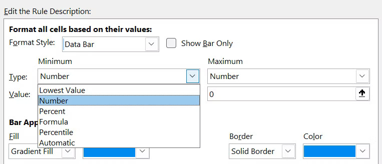
This is where things get interesting and a little less obvious. Excel creates data bars by comparing each cell's value to other cells in the range you've selected. The software automatically sets the minimum and maximum values based on the range of values you've selected.

This means that if your data ranges from 30 to 90, Excel will set 30 as the smallest bar and 90 as the longest bar. However, if you apply the same format to another column with a different range (say, 0 to 50), a value like 45 might look longer than 60 in the first set.

To keep things consistent, you should manually set the minimum and maximum values. Go to Edit Rule , then under Minimum and Maximum , select Number and enter fixed values (like 0 and 100).

Another oddity is that blank cells, zeros, and negative numbers behave in slightly different ways.

1. Empty cells do not display any bars.
2. The zeros create a small gradient, which looks like a small value.
3. Negative numbers create bars in the opposite direction (to the left). By default, they also have a different fill color, although you can modify this by clicking Negative Value and Axis… .
4. Even identical values can appear unequal if decimals are used.

To avoid these and any other problems, you can apply the following tips:

1. Round data before applying formatting.
2. Replace spaces with placeholder characters like 0 or "N/A" if they are not visually designed to be blank.
3. Data bars only work with numeric values, so Excel will ignore these values.
4. For large spreadsheets, consider applying data bars only to summary or key figures rather than individual data points. Large data sets can slow down Excel's responsiveness when using data bars, since it has to recalculate the bar length every time the value changes.

Data bars won't replace everything with charts, but when you want a quick, visual way to integrate right into your spreadsheet, they're perfect. They keep your layout clean, show insights instantly, and impress your audience, even if they don't realize what's changed.

David Pac

Update 05 August 2025