MS Excel 2007 - Lesson 14: Layout

TipsMake.com - Split spreadsheet

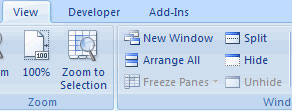
In Excel 2007, you can split a spreadsheet into multiple regions to easily view each section of a spreadsheet. To separate spreadsheets:

• Select the central cells of the spreadsheet you want to split

• Click the Split button on the View tab

• The screen separation notice appears, you can manipulate each section separately.

MS Excel 2007 - Lesson 14: Layout Picture 1

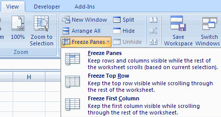
Making freezing rows and columns

You can select a specific part of a spreadsheet to keep it unchanged while working with other sections. This is done through the Freeze Rows and Columns feature (freezing rows and columns):

• Click the Freeze Panes button on the View tab

• Select a part to freeze or click at the beginning of each column or left side of the line

• To cancel the freeze application, click the Freeze Panes button

• Click Unfreeze

MS Excel 2007 - Lesson 14: Layout Picture 2

Hide the spreadsheet

To hide spreadsheet:

• Select the sheet tab that you want to hide

• Right-click on that tab

• Click Hide

MS Excel 2007 - Lesson 14: Layout Picture 3

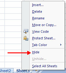
To cancel hidden spreadsheet:

• Right click on any spreadsheet

• Click Unhide

• Select a spreadsheet to cancel hiding.

MS Excel 2007 - Lesson 14: Layout Picture 4