How to use the MROUND function in Excel

Unlocking the power of Excel's MROUND function will give you precision in your calculations. Here's what you need to know about the MROUND function in Microsoft Excel .

How to use the MROUND function in Excel Picture 1

Excel is a repository of many functions and formulas. Each function serves a specific purpose to help you perform complex tasks efficiently. Among these functions, MROUND stands out as a valuable tool for achieving computational accuracy. Now let's explore how to use the MROUND function in Excel and practice through some real-life examples.

What is the MROUND function in Excel?

The MROUND function in Excel is used to round a number to the nearest multiple of a specific value. Its syntax is quite simple:

=MROUND(number, multiple)

In there:

1. Number is the value you want to round to the nearest multiple.
2. Multiple is the set of numbers that you want to round.

Examples of how to use the MROUND function in Excel

Round to the nearest integer

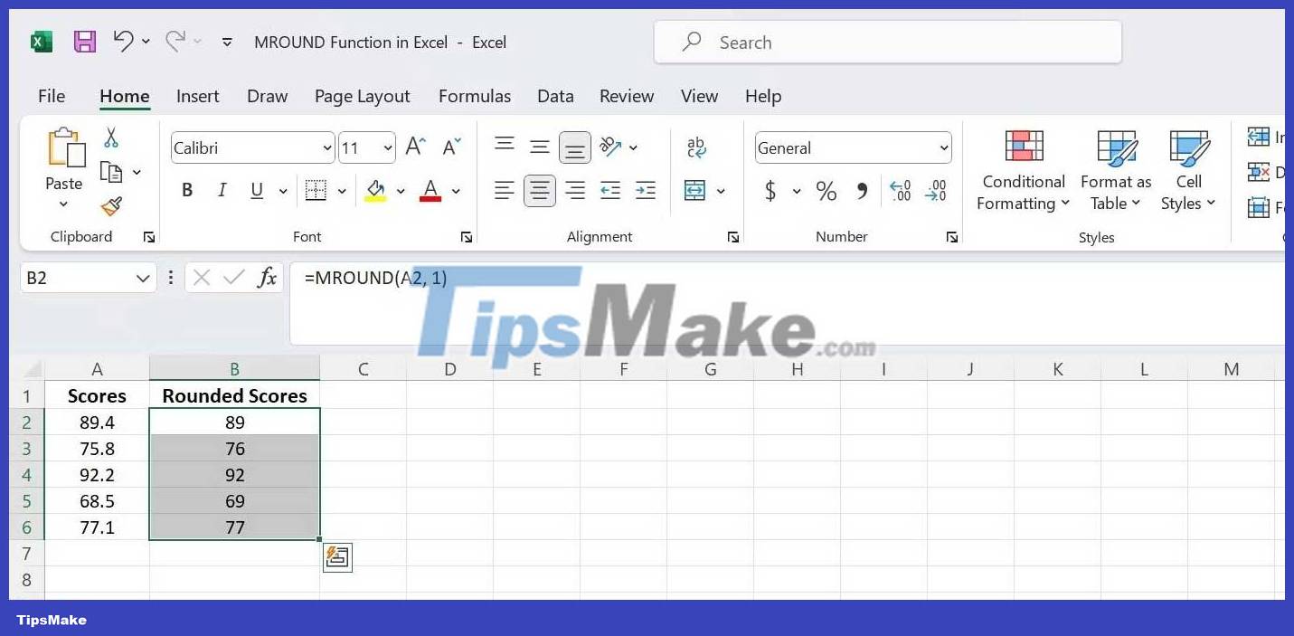
Suppose you have a list of students' test scores with decimal values ​​and want to round each number to the nearest value. You can use the MROUND function to achieve this quickly:

=MROUND(A2, 1)

How to use the MROUND function in Excel Picture 2

This formula will remove the decimal part of the number in A2 and round it to the nearest number.

Round to the nearest multiple

Suppose you have a list of prices in column A, and want to round each price to the nearest multiple of $5. The MROUND formula below is as follows:

=MROUND(A2, 5)

This will round the value in cell A2 to the nearest multiple of 5.

How to use the MROUND function in Excel Picture 3

Round the time value

For datasets containing times, rounding them to the nearest 15-minute block can be achieved by entering the following formula:

=MROUND(A2, "0:15")

How to use the MROUND function in Excel Picture 4

Here, "0:15" is the multiple to which you want to round the time value. In this case, 0:15 represents 15 minutes, indicating that you want to round the time to the nearest 15-minute increment or interval.

Round negative numbers

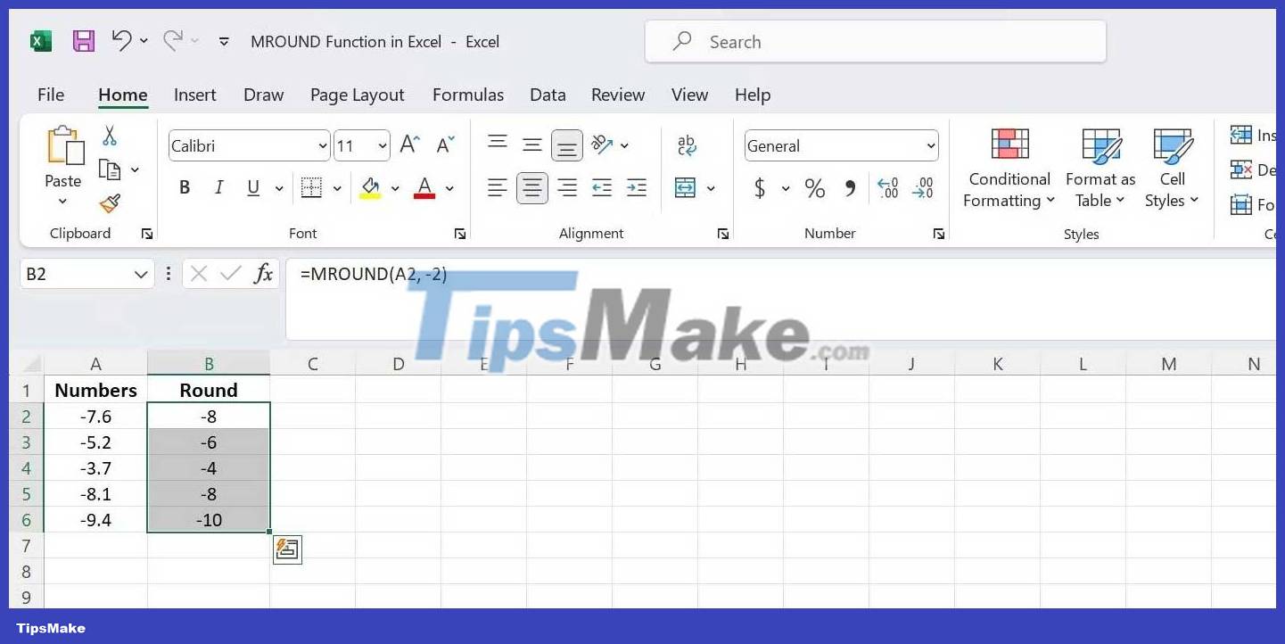
The MROUND function can also handle negative numbers. To round a negative number to the nearest multiple, use a negative value for the multiple argument. For example:

=MROUND(A2, -2)

How to use the MROUND function in Excel Picture 5

This will round the negative number in cell A2 to the nearest multiple of -2.

How to use MROUND with other Excel functions

Excel functions show their true power when combined with other functions, and MROUND is no exception. Here's an example of how to use MROUND with other functions:

Use MROUND with SUM

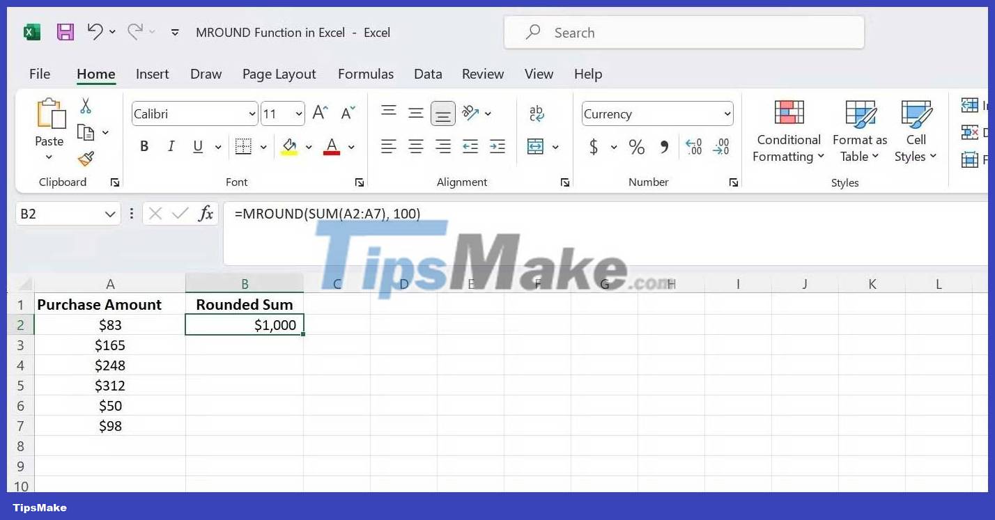
Suppose you have a list of purchase quantities in column A, and want to calculate the total quantity, rounding to the nearest 100USD. You can use the SUM function with MROUND to do this:

=MROUND(SUM(A2:A7),100)

This sums the range of values, then rounds the result to the nearest multiple of 100.

How to use the MROUND function in Excel Picture 6

Use MROUND with IF

Suppose you have a list of test scores in column A, and you want to round a number greater than or equal to 60 to the nearest 10. You can use the IF function with MROUND as follows:

=IF(A2 >= 60, MROUND(A2, 10), A2)

This formula checks the score in cell A2 to see if it is greater than or equal to 60. If so, it rounds the score to the nearest multiple of 10 using MROUND. Otherwise, it will keep the same score.

How to use the MROUND function in Excel Picture 7

By combining MROUND with other functions, you can process calculations to meet specific requirements, ensuring accuracy in results.

Marvin Fry

Update 27 October 2023