How to use the Match function in Excel

The Match function in Excel is a function that searches a predetermined value in a cell range and returns the relative position of the value in that range.

Match is a common function in Excel functions , which is used quite a lot when processing Excel data tables and calculations. In a data table, when you want to search for a certain value in an array, or cell range, the Match function returns exactly the position of that value in the array or in the range of the data table. .

This helps users quickly find the value they need, without having to search manually, especially with multiple tables of data that will take time. The following article will show you how to use the Match function in Excel.

The Excel function syntax is: = Match (Lookup_value, Lookup_array, [Match_type]).

Inside:

1. Lookup_value: search value in Lookup_array array. This value can be a number, text, logical value, or a cell reference to a number, text, or logical value, required.
2. Lookup_array: array or range of cells to be searched, required.
3. Match_type: search type, not necessarily.

There are 3 types of search in Match function on Excel:

1. 1 or omitted (Less than): The Match function searches for the largest value that is less than or equal to lookup_value. If the user chooses this type of search, lookup_array must be sorted in ascending order.
2. 0 (Exact Match): The Match function will search for the first value exactly with lookup_value. Values ​​in lookup_array can be sorted by any value.
3. -1 (Greater than): The Match function finds the smallest value that is large or equal to lookup_value. The value in lookup_array must be sorted in descending order.

Note when using the Match function:

1. The Match function returns the position of the search value in lookup_array, not returning the search value itself.
2. You can use uppercase or lowercase letters while searching for text values.
3. When the search value cannot be found in lookup_array, the Match function will report a search value error.
4. In case the Match_type is 0 and the lookup_value search value is text, the search value may contain * (for strings) and question marks (for single characters). If you want to find a question mark or a star, type the tilde before that character.
5. If you don't enter anything, the default Match function is 1.

Example 1:

We will take the example with the total table of products below.

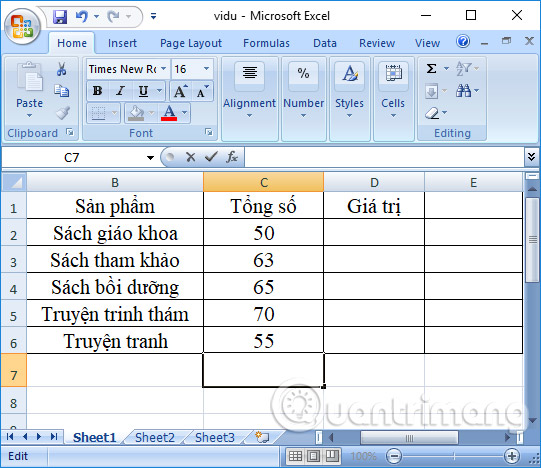
Case 1: Search type is 1 or omitted

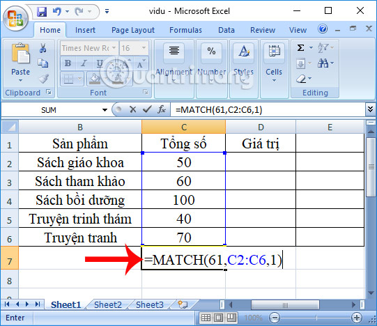
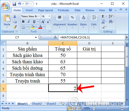
Search for the number 61 in the Total column in the data table, ie search for a value less than the search value. We enter the formula = = MATCH (64, C2: C6,1) .

Since the value 64 is not in the Total column, the function returns the position of the closest small value whose value is less than 64 is 63. The result will return the value in the second position in the column.

Case 2: Search type is 0

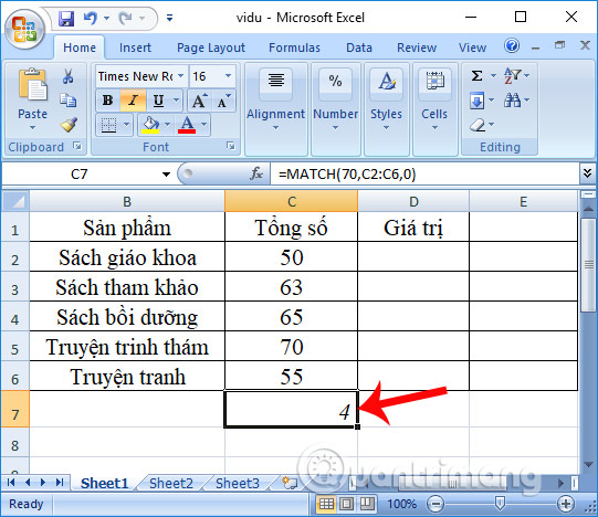
Search for the position of value 70 in the data table. We will have the input formula = MATCH (70, C2: C6,0) and press Enter.

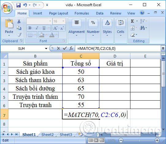
The returned result will be the position of the value 70 in the Total column is the 4th position.

Case 3: The search type is -1

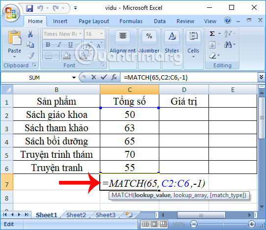
We will have the formula = MATCH (65, C2: C6, -1) as shown below.

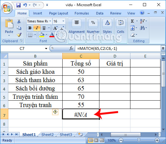
However, because the array is not sorted in descending order, it will report an error as shown below.

Example 2:

For the student group data sheet below. Find students' class order in this data sheet, with the order given below.

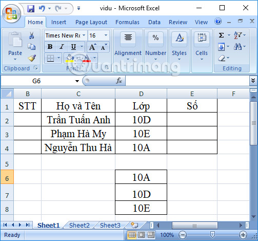
The order search formula is = MATCH (D2, $ D $ 6: $ D $ 8.0) and then press Enter.

Immediately after that, the returned result will be the exact order of the students in each class, arranged according to the rules given.

The above are examples as well as detailed cases using the Match function on Excel. With this function, users can search for the exact location of the value within the search range, or rearrange the order without having to do it manually.

I wish you all success!