How to Use the MATCH Function and Combine the MATCH Function

This updated guide explains how to Use the MATCH Function and Combine the MATCH Function through clear steps, practical examples, and important checks that help prevent common errors.

1. How to Use the MATCH Function in Excel

The MATCH function in Excel is used to search for a given number in a list

a) The syntax of the MATCH function

MATCH (Lookup_value, Lookup_array, [Match_type])

Arguments

- Lookup_value: Search value, can be a numeric value, text, logical value or a cell reference to a number, text or logical value, required

- Lookup_array: Array to search, required

- Match_type: Search type. Optional.

There are 3 types of search:

+ 1: Less than (Less than the search value)

+ 0: Exact match (Exact match value)

+ 1: Greater than (greater than the search value)

When omitting nothing, the default MATCH function is 1

b) Illustrative example

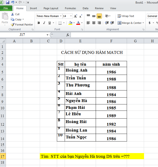
Give the following list of students. Find the student serial number named Nguy?n H�

Use the MATCH Function and Combine the MATCH Function � Arguments screenshot 1

Step 1:

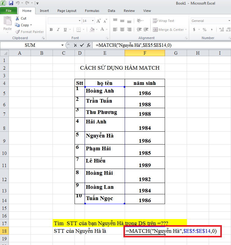
In cell F18, you will enter the formula according to the above syntax, and then we press Enter to perform the MATCH function

F18 = MATCH ('Nguyen Ha', $ E $ 5: $ E $ 14,0)

Use the MATCH Function and Combine the MATCH Function � Arguments screenshot 2

Step 2:

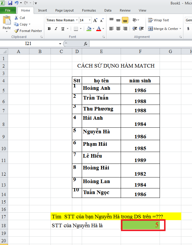
Soon we will be returning the value of position F18 as the number '5'

Use the MATCH Function and Combine the MATCH Function � Arguments screenshot 3

2. How to Combine INDEX and MATCH Functions

People often use the MATCH and INDEX functions to find a certain value. Because index searches only when it knows the row and column addresses in the worksheet area.

Therefore match acts as a search for the position of the row and column of the value to be searched.

Here, to better understand how to combine, let's find out through the example below:

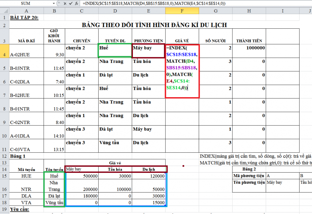
Give 2 tables as examples in the image. Please fill in the ticket price corresponding to the route code and transportation

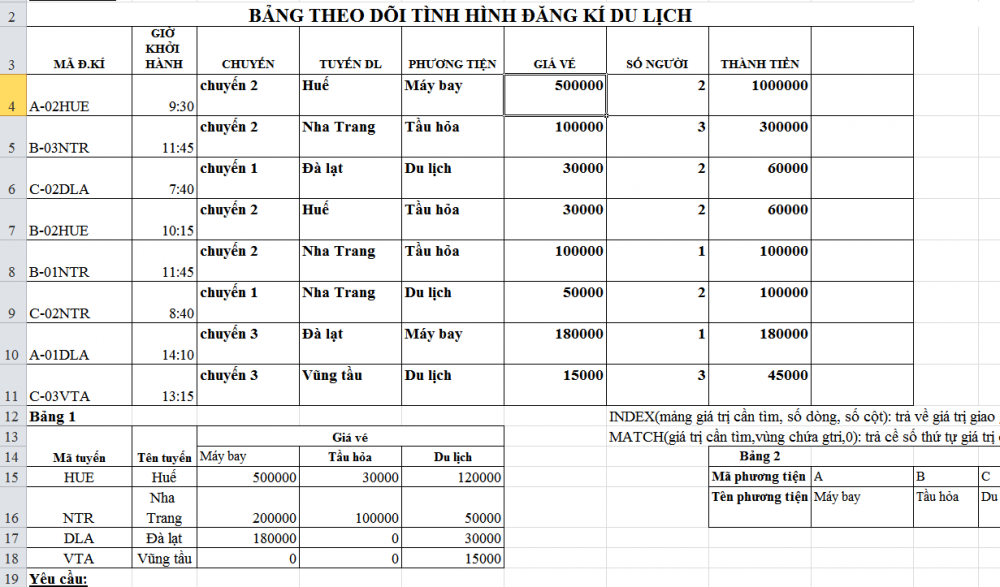
Use the MATCH Function and Combine the MATCH Function � 2. How to Combine INDEX and MATCH Functions screenshot 4

Step 1: In cell F4, you will enter the formula with the syntax = INDEX ($ C $ 15: $ E $ 18, MATCH (D4, $ B $ 15: $ B $ 18,0), MATCH (E4, $ C $ 14: $ E $ 14,0)) and then we press Enter to execute the MATCH function

Use the MATCH Function and Combine the MATCH Function � 2. How to Combine INDEX and MATCH Functions screenshot 5

Step 2:

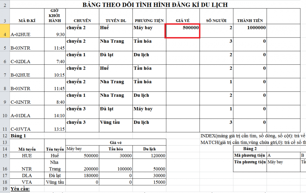
Soon we will be returned to the F4 position value of 500000

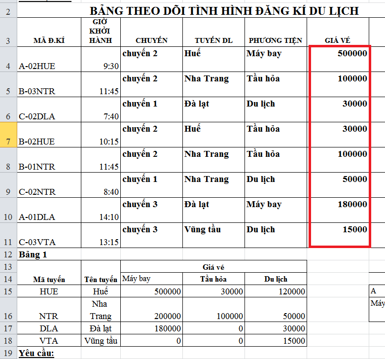
Use the MATCH Function and Combine the MATCH Function � 2. How to Combine INDEX and MATCH Functions screenshot 6

We then drag the formula to complete the worksheet and get the following result table

Use the MATCH Function and Combine the MATCH Function � 2. How to Combine INDEX and MATCH Functions screenshot 7

The jaw looks very long but actually it's not that hard right? We just need to understand the nature and usage of functions to be flexible and combined to handle difficult Excel exercises. Good luck!

social shareand social share

FAQ

What is the easiest way to Use the MATCH Function and Combine the MATCH Function?

Start with the requirements in this guide, then follow each step in order. Check the result after every major change so problems are easier to identify.