How to rank on Excel with RANK function
To rank on Excel we will use the RANK function. You can rank in ascending or descending order according to your needs.
When working with the statistics table on Excel need to classify rankings, the survey grows, we need to use the RANK function. RANK function will help you rank data to know which data is high and low. Users using RANK function can rank in order from high to low or from low to high. Using RANK function is also relatively easy as other basic Excel functions. The following article will guide you how to use RANK function on Excel.
- How to use the SUM function to calculate totals in Excel
- How to combine Vlookup function with If function in Excel
- How to automatically display names when entering code in Excel
Instructions for using RANK function on Excel
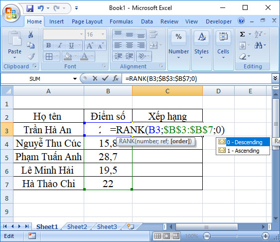
We will apply to the score table below with the requirement to rank the score in with the RANK function.
The function RANK has the formula = RANK (number, ref, [order]) .
- Number: The value to rank in the block.
- Ref: List, data block to be sorted.
- Order: Sort order, sort type (ascending or descending). In the case of order = 0 (or without this parameter), it will be calculated from high to low. And order = 1 will rank from low to high.

1. Sort from high to low
Step 1:
In the first cell in the Ranking column, enter the formula = RANK (B3, $ B $ 3: $ B $ 7.0) .
Inside:
- B3 is the number to look for in the rankings as the first student's score.
- $ B $ 3: $ B $ 7 is the number list that is the Score column.
- 0 is sorted in ascending order (the highest score will rank 1).

Step 2:
After pressing Enter they will have a result of 3, meaning that Tran Ha An is ranked 3rd with 20.1 points. In the first result box in the Ranking column, you scroll down to the remaining cells and get the ranking results for the others.
In case of overlapping numbers, there will be equal rankings and affect rankings later. For example, the number 22 will appear twice, it will rank 2. And the number 20.1 will rank 4th always and there is no 3rd rank.

2. Sort from low to high
In this case it needs to be reversed, meaning that those with a high score will rank at the bottom of the list. Here we will replace 0 to 1.
We will also enter the formula in the first rank cell = RANK (B3, $ B $ 3: $ B $ 7.1) and then press Enter.

The result will also be as shown below.

So you know how to use RANK function in Excel to rank data, from high to low or from low to high. Using RANK function will save more time to find the highest, or lowest, data than manual number detection.
Video tutorial using RANK function on Excel
See more:
- 4 basic steps to color alternating lines in Microsoft Excel
- Summary of expensive shortcuts in Microsoft Excel
- How to keep Excel and Excel columns fixed?
I wish you all success!
- How to use the RANK function in Excel
- RANK.AVG function - The function returns the rank of a number in a list of numbers in Excel
- PERCENTRANK function - The function returns the rank of the value in Excel
- RANK.EQ function - Function returns the rank of a number in a list of numbers, returns the highest rank when multiple values with the same rank in Excel
- PERCENTRANK.INC function - The function returns the rank of a value in a dataset as a percentage including values 0 and 1 in Excel
- PERCENTRANK.EXC function - The function returns the rank of a value in a dataset as a percentage excluding values 0 and 1 in Excel


 How to use the RANK and SUMPRODUCT functions in Excel with COUNTIF
  How to calculate rank for season 1 and how to check rank Dota Auto Chess
  League of Legends: 6 tips to help you climb rank quickly
  PERCENTRANK.INC function - The function returns the rank of a value in a dataset as a percentage including values 0 and 1 in Excel
  RANK.EQ function - Function returns the rank of a number in a list of numbers, returns the highest rank when multiple values with the same rank in Excel
  RANK function - Rank function in Excel - Usage and examples