How to Use the RANK Function in Excel: Step-by-Step Guide

This updated guide explains how to Use the RANK Function in Excel through clear steps, practical examples, and important checks that help prevent common errors.

Those who are new to Excel functions may not know the syntax and usage of the Rank function. this guide describes the function, syntax and usage of the Rank function in Excel.

Description

The Rank function returns the rank of a number in a list of numbers, the rank of a number is its value rank compared to other values in the list of numbers. It is similar to data sorting but has superior results and is easier to manage.

Syntax

RANK (number, ref, [order])

Arguments

- number: the number you may need to find the rank.

- ref: array or reference to a list of numbers, if the value is not a number, it will be ignored.

- order: sort order (ascending or descending). If the order is 0 (or no parameters) then the result will be sorted descending. If the order is 1 or any value other than 0, the result will be ascending.

For Example

For the following data sheet, a ranking of employees is required based on the number of products sold. The employee who sells the most products will rank first.

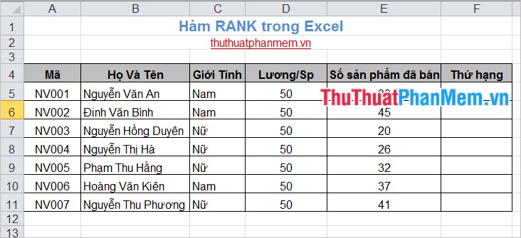
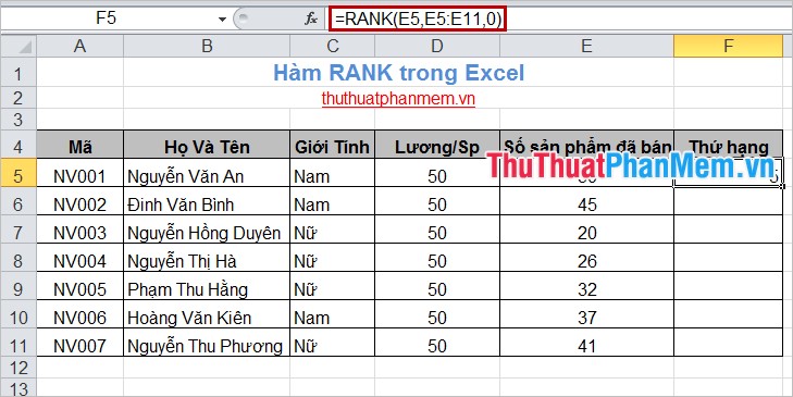
First, you need to write the RANK function formula for the ranking cell in cell F5:

= RANK (E5, E5: E11,0)

Arguments

E5 is the number to find (rank of product sold by the first employee).

E5: E11 is a list of numbers (in the example, a list of products sold by all employees who need to be ranked).

0 is sorted in ascending order (the highest number of products sold will rank as 1).

The following results:

Enter the formula with the remaining cells, replace the number to find the rank corresponding to the formula position and keep the list of numbers and sort order. The result will get the following:

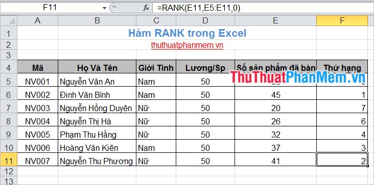
With identical numbers there will be equal rank but affect the rank after it. For example, the number 15 appears twice and has a rank of 6, then the number 16 will have a rank of 8 (no number with a rank of 7). So, you already know the function, syntax and usage of the Excel Rank function. To understand and master the Rank function, you need to use the Rank function more often. Good luck!