How to convert negative numbers to positive numbers Excel

When presenting or editing spreadsheet data in Excel, you need to convert negative numbers into positive numbers or vice versa from positive numbers to negative numbers. If making a manual switch to delete each negative sign is only appropriate when the Excel table has little data, there are many columns of data, this approach is not feasible. In fact, to convert negative numbers to positive numbers, or vice versa on Excel is very simple without using complicated Excel functions. The following article will guide you how to convert negative numbers to positive numbers and vice versa on Excel.

1. Instructions to stamp negative numbers in Excel
2. Instructions for separating column content in Excel
3. How to convert money into words in Excel
4. How to display 0 in front of a number in Excel

How to 1. Change the number to positive numbers with Paste Special

For example, I have the Excel data table below with a negative number like the image.

Step 1:

First of all, enter the -1 number into any empty cell on the Excel table.

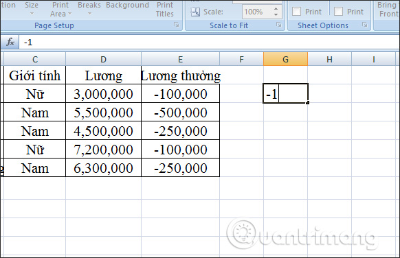
Step 2:

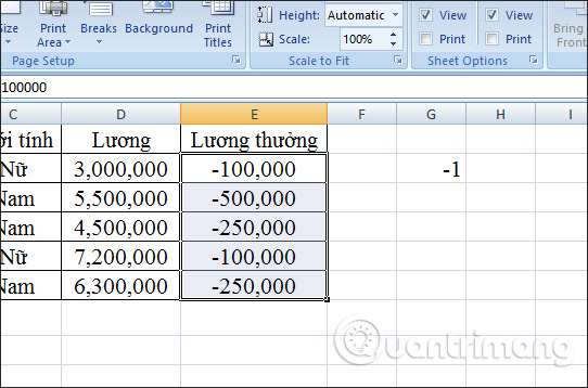
Then click copy this -1 and then black out all negative numbers to convert to positive numbers. If there is a negative number in each position, then press Ctrl and click on each of them, select the right mouse button.

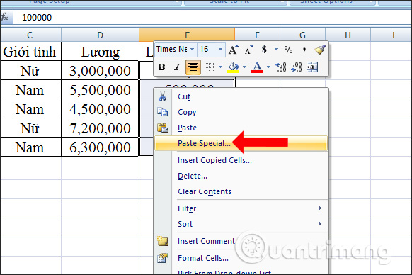
Right-click and choose Paste Special or click the arrow at the Paste button on the Home tab of the ribbon bar, then also select Paste Special.

Step 3:

Display the new dialog interface and click on Multiply and click OK as shown.

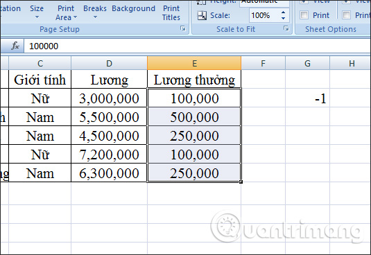
The entire negative number column has been converted to positive numbers with a very fast way.

Method 2: Use the IF function to convert negative numbers to positive

In case your data column has many positive and negative numbers alternating with each other, but you want to change negative numbers to positive numbers, you can use the IF function.

Step 1:

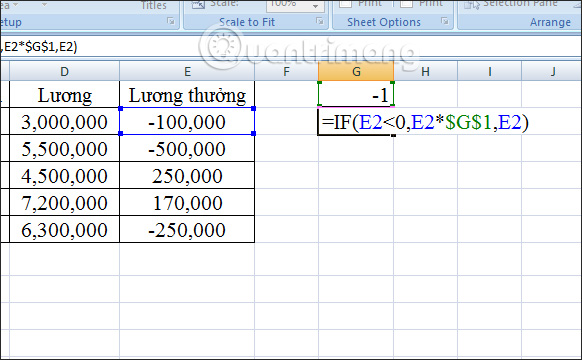
We have the data table below and also enter the number -1 at any position you want.

Step 2:

In cell G3, enter the formula = IF (E2 <0, E2 * $ G $ 1, E2). In which, if the value of cell E2 is less than 0, multiply by G1, if the value is greater than 0, remain the same.

Step 3:

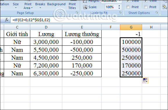
Press Enter and see the value converted to positive numbers. Clicking on the box and then dragging down the remaining cells will display the results as shown.

Step 4:

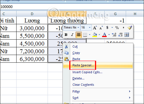
Copy all the data from G2 to G6 and black out the column E2 to E6 and right-click and choose Paste Special , or click the arrow in the Paste button on the Home tab of the menu bar, then select Paste Special.

Step 5:

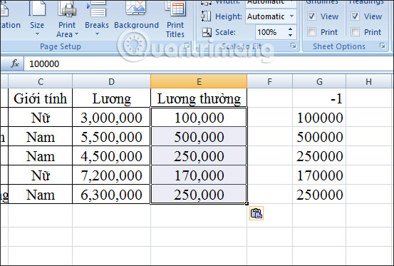
In the display interface, click on Values and click OK.

Immediately the value in G2 to G6 column has shifted to column E2 to E6 as shown.

2 ways to convert negative numbers to positive numbers or vice versa on Excel are very simple. For the second way, the IF function automatically filters out values ​​less than 0 to multiply by -1, if the data column mixes two types of numbers together. Depending on how your data column is, we choose the appropriate usage.

I wish you all success!