This Excel trick will end the pain of resizing tables!

Nothing ruins your workflow like inserting new data and realizing your Excel table isn't big enough. Everyone used to have to drag the edges until they learned this simple trick to make their Excel table expand on its own.

 

Dynamic Arrays are the right way to expand Excel tables

Instead of returning a single value, dynamic arrays spill the result across multiple cells without requiring you to specify the exact range first. This behavior makes them suitable for creating self-expanding tables.

Examples include the UNIQUE , SORT , and FILTER functions . These functions return dynamic arrays that can expand or shrink based on your source data. As you add new items to the dataset, the results are updated immediately without any manual intervention.

When you enter a dynamic array formula into a cell, Excel automatically fills the adjacent cells necessary to display all the results. You'll know it's working when you see a blue border around the range. Trying to enter something in this spill area will result in a #SPILL! error , which is a helpful warning.

Using dynamic arrays is not only convenient but also reliable, as manual table management can lead to errors, missing data, and frustration.

How to create a self-expanding list for unique items

The UNIQUE function is one of those functions that can save you a lot of work. Instead of manually scanning through lists, use this function to automatically extract unique values from your data.

Here is the basic syntax:

=UNIQUE(array, [by_col], [exactly_once])

The array parameter contains the source data, such as a column of employee departments or customer names. The by_col parameter (TRUE or FALSE) specifies whether to compare by column or row, while exactly_once filters for values that appear only once.

 

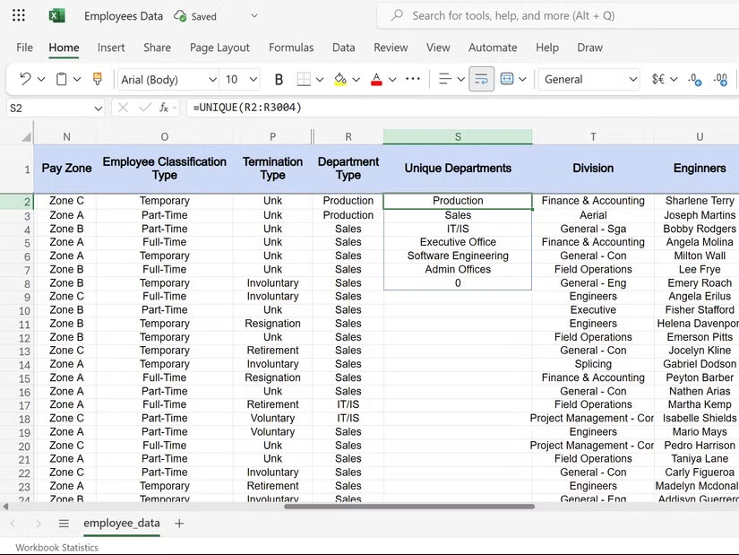
Let's say you're working on an employee data spreadsheet and need a list of all departments, just type:

=UNIQUE(R2:R3004)

Here, column R contains department names from rows 2 to 3004. Excel will instantly create a dynamic list of unique departments, which will be updated every time a new person joins the team.

This method is also superior to traditional Excel duplicate removal methods because dynamic arrays remain connected to your source data. Manual duplicate removal, on the other hand, creates static lists that become outdated as soon as you add new items.

For exact_once cases , you can use the following formula to find departments with only one employee. This formula is effective in identifying understaffed groups or unique roles in your organization.

=UNIQUE(R2:R3004,,TRUE)

You can also automatically sort your dynamic lists.

The SORT function takes dynamic arrays to the next level. Continuing with the employee data example, instead of manually sorting employee names or salary data, Excel automatically handles the sorting whenever the data changes. Here is the syntax for the SORT function:

 

=SORT(array, [sort_index], [sort_order], [by_col])

The array parameter contains the range of data, sort_index specifies the column to sort by, sort_order specifies ascending (1) or descending (-1), and by column specifies whether to sort by column (TRUE) or by row (FALSE).

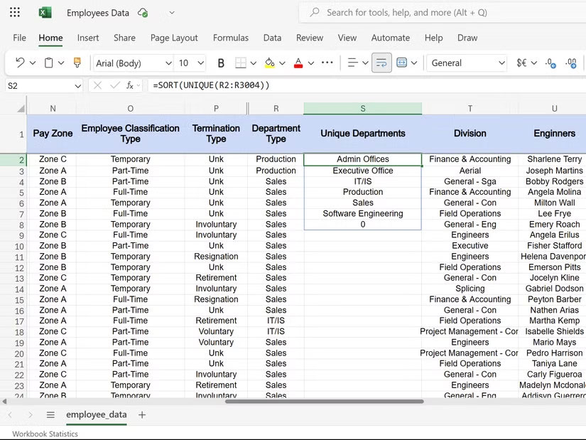
The SORT function can be combined with the UNIQUE function for better results. For example, the following formula will return a list of unique departments sorted alphabetically from a list of employees. When HR adds new departments, they will automatically appear in the correct alphabetical position.

=SORT(UNIQUE(R2:R3004))

If we need to analyze salaries, we can use:

=SORT(A:H, 8, -1)

The above formula sorts the employee data by salary in descending order. The 8th column contains the salary, and -1 sorts from highest to lowest.

Note : The SORT function is case sensitive and treats numbers stored as text differently than real numbers. Make sure the data types are consistent to sort correctly.

You can see the Excel SORT function tutorial for more examples. The goal is to automate the update, so that sorted lists are refreshed instantly without any manual intervention.

The FILTER function is the top choice for dynamic reports.

If you've never used Excel's FILTER function, you're really missing out. The FILTER function creates one of the most powerful dynamic reports. You can use it to automatically display only data that meets your criteria without creating static copies that will eventually become outdated.

The syntax of the Filter function is:

=FILTER(array, include, [if_empty])

array contains your entire dataset, include defines your criteria, and if_empty displays a custom message when no results match the condition.

 

People frequently use this function for various reports. For example, if we want to display all the members of the sales team from the employee database, we can use it in the following way:

=FILTER(A:Q, Q:Q="Sales")

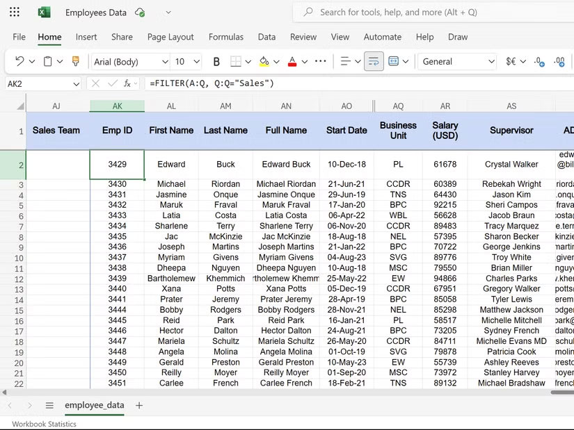
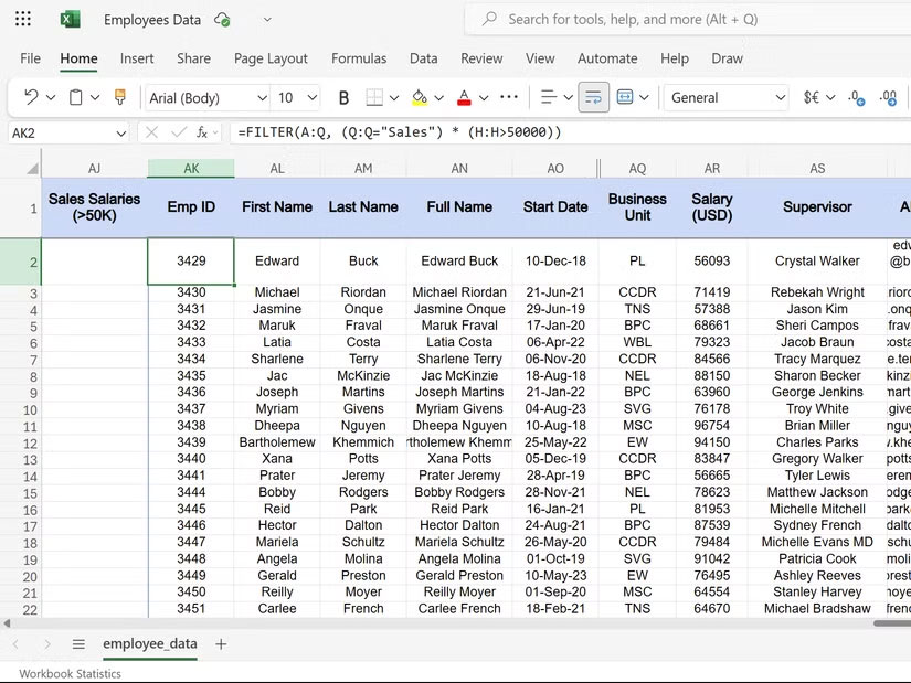
When someone moves to the sales department, they will automatically appear in the filtered results. Similarly, to analyze salaries, we can use the following formula to show employees who earn over $50,000.

=FILTER(A:H, H:H>50000)

If someone gets a raise, they will suddenly appear in this high income report. Additionally, we can also combine criteria:

=FILTER(A:Q, (Q:Q="Doanh số") * (H:H>50000))

The formula above shows sales team members who earned more than $50,000. The asterisk (*) acts as an AND operator, requiring both conditions to be true.

Tip : FILTER returns the #CALC! error if no results match the criteria. Use the if_empty parameter to display "No results found".

Dynamic arrays are useful because they eliminate manual table updates and eliminate missing entries. Excel becomes more intuitive when you start using UNIQUE, SORT, and FILTER together.