Match function in Excel: How to use the Match function with examples

The Match function in Excel has many practical applications. Below are details on how to use the Match Excel function .

The Match function is a popular function in Excel functions, used a lot when processing Excel data tables and calculations. In a data table, when you want to search for a certain value in an array or cell range, the Match function will return the correct position of that value in the array or within the range of the data table. .

This helps users quickly find the value they need, without having to search manually, especially with tables with lots of data, which would be time-consuming. The article below will guide you how to use the Match function in Excel .

Match function syntax in Excel

The syntax of the Match function in Excel is: =Match(Lookup_value,Lookup_array,[Match_type]).

In there:

1. Lookup_value: search value in Lookup_array array. This value can be a number, text, logical value, or a cell reference to a number, text, or logical value, which is required.
2. Lookup_array: array or cell range to be searched, required.
3. Match_type: search type, not required.

There are 3 types of searches in the Match function in Excel:

1. 1 or omitted (Less than): the Match function searches for the largest value that is less than or equal to lookup_value. If the user selects this type of search, the lookup_array must be sorted in ascending order.
2. 0 (Exact Match): the Match function will search for the first value that is exactly equal to lookup_value. The values ​​in lookup_array can be sorted by any value.
3. -1 (Greater than): Match function searches for the smallest value that is greater than or equal to lookup_value. Values ​​in lookup_array must be sorted in descending order.

Note when using the Match function:

1. The Match function returns the position of the lookup value in lookup_array, not the lookup value itself.
2. You can use uppercase or lowercase letters while searching for text values.
3. When the search value cannot be found in lookup_array, the Match function will report a search value error.
4. In case Match_type is 0 and the lookup_value search value is text, the search value can contain * characters (for character strings) and question marks (for single characters). If you want to find a question mark or asterisk, type a tilde before that character.
5. If nothing is entered, the default Match function is 1.

Types of MATCH functions in Excel

Here are the different types of MATCH functions in Excel:

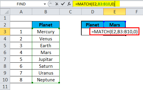
1. Exact match

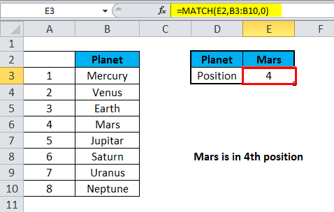
The MATCH function performs an exact match when the match type is set to 0. In the example below, the formula in E3 is:

=MATCH(E2,B3:B10,0)

Match function in Excel: How to use the Match function with examples Picture 1

The MATCH function returns an exact match of 4.

Match function in Excel: How to use the Match function with examples Picture 2

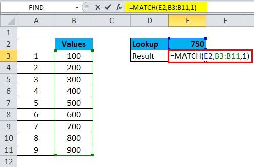
2. Approximate match

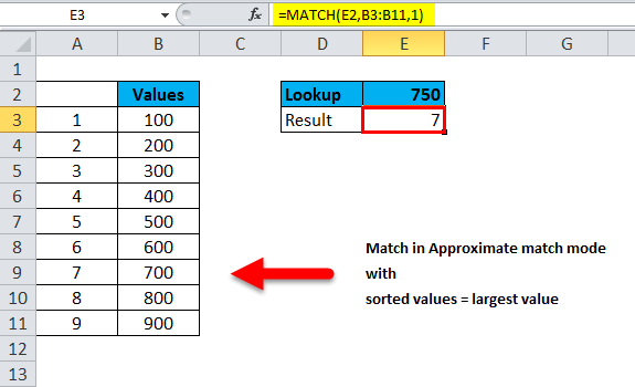
MATCH will perform an approximate match on values ​​sorted from AZ when the match type is set to 1, finding the largest value that is less than or equal to the lookup value. In the example below, the formula in E3 is:

Match function in Excel: How to use the Match function with examples Picture 3

The MATCH function in Excel returns an approximate match of 7.

Match function in Excel: How to use the Match function with examples Picture 4

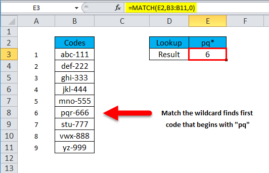
3. Wildcard matching

The MATCH function can perform wildcard matching when the match type is set to 0. In the example below, the formula in E3 is:

Match function in Excel: How to use the Match function with examples Picture 5

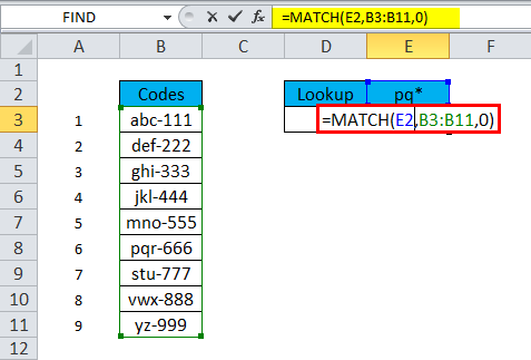
The MATCH function returns the result of the wildcard character 'pq'.

Match function in Excel: How to use the Match function with examples Picture 6

Note:

1. The MATCH function is not case sensitive.
2. Match returns the #N/A error if no match was found.
3. The lookup_array argument must be in descending order: True, False, ZA,…9,8,7,6,5,4,3,…, etc.
4. You can find wildcard characters like asterisks and question marks in lookup_value if match_type is 0 and lookup_value is in text format.
5. Lookup_value can have wildcards such as asterisks and question marks if match_type is 0 and lookup_value is text. The asterisk (*) matches any type of character string; Any single character is matched by a question mark (?).

4. How to apply Index and Match in an Excel formula

Match and Index when combined together will give you many benefits. For example, calculate revenue and profit from any application from the provided database. Here's how you can do this:

1. Open the INDEX function.

2. Select cells C3:C13 as the revenue data source (Revenue).

Match function in Excel: How to use the Match function with examples Picture 7

3. Enter MATCH and press Tab .

4. Select G2 as the lookup value, B3:B13 as the source data, and 0 for a complete match.

Match function in Excel: How to use the Match function with examples Picture 8

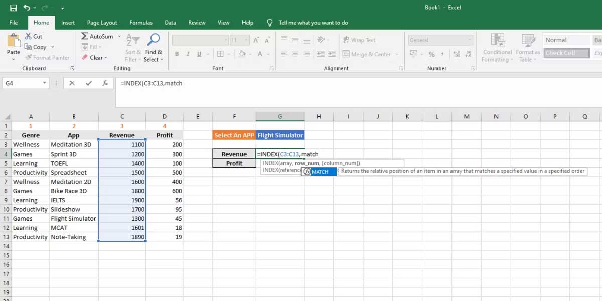
5. Press Enter to fetch information for the selected application.

6. Follow the steps above and replace the INDEX source with D3:D13 to get Profit .

Match function in Excel: How to use the Match function with examples Picture 9

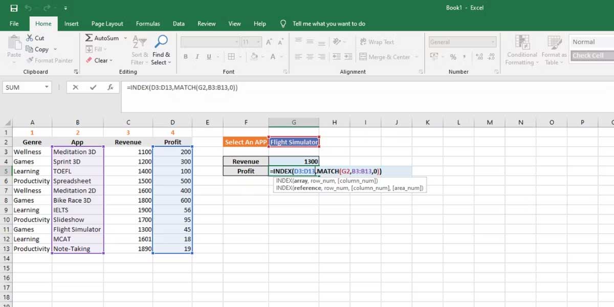
7. Now this formula will be implemented in Excel:

=INDEX(C3:C13,MATCH(G2,B3:B13,0)) =INDEX(D3:D13,MATCH(G2,B3:B13,0))

Above is an example of one-way use of INDEX MATCH in Excel. You can also select rows and columns to perform more complex searches.

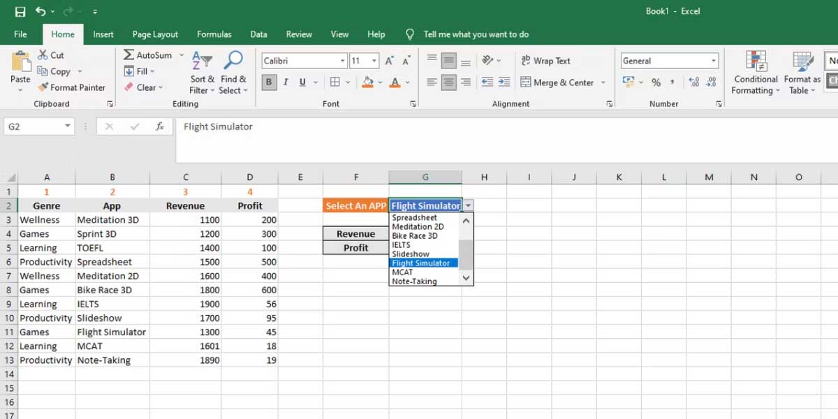
For example, you can use a drop-down menu instead of separating cells for Revenue and Profit. You can follow these steps to practice:

1. Select the Revenue box and click the Data tab on the ribbon.

2. Click Data Validation and under Allow , select List .

Match function in Excel: How to use the Match function with examples Picture 10

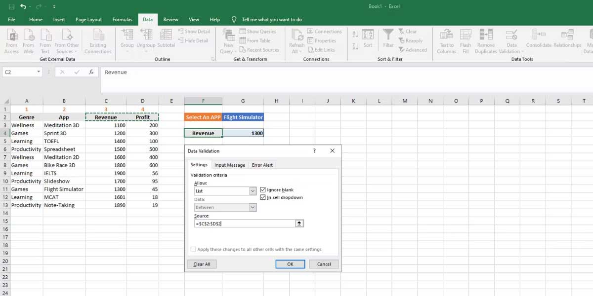
3. Select the Revenue and Profit column heading as Source .

4. Click OK .

Match function in Excel: How to use the Match function with examples Picture 11

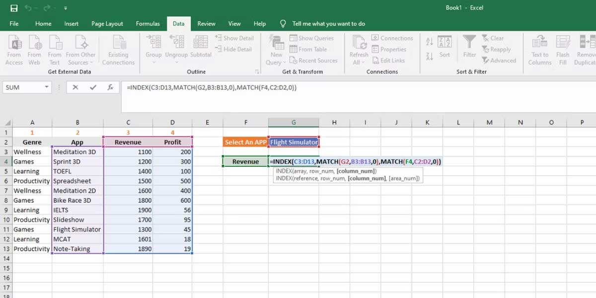
5. In this formula, you use the MATCH function twice to fetch both row and column values ​​for the final INDEX function.

6. Copy & paste the following formula next to the Revenue cell to get the value. Just use the drop-down menu to choose between Revenue and Profit.

=INDEX(C3:D13,MATCH(G2,B3:B13,0),MATCH(F4,C2:D2,0))

Match function example

Example 1:

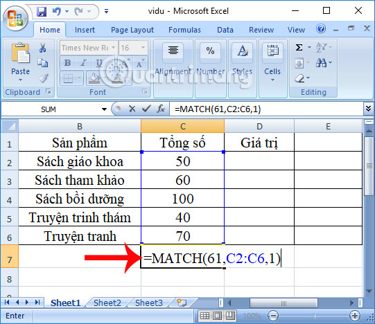
We will take an example with the total number of products table below.

Match function in Excel: How to use the Match function with examples Picture 12

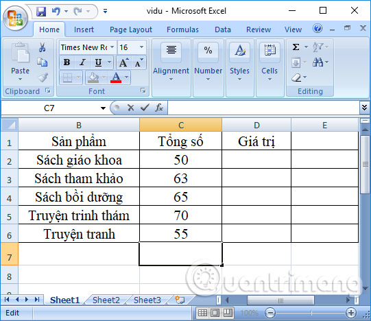
Case 1: Search type is 1 or omitted

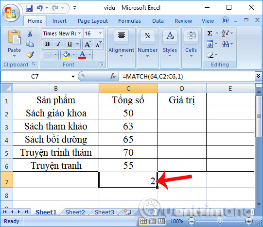
Search for position number 61 in the Total column in the data table, meaning search for a value smaller than the search value. We enter the formula =MATCH(64,C2:C6,1) .

Match function in Excel: How to use the Match function with examples Picture 13

Because the value 64 is not in the Total column, the function will return the position of the nearest small value whose value is less than 64, which is 63. The result will return the value in the 2nd position in the column.

Match function in Excel: How to use the Match function with examples Picture 14

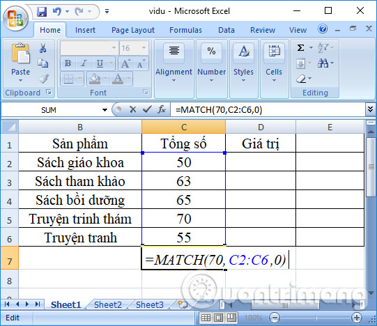
Case 2: Search type is 0

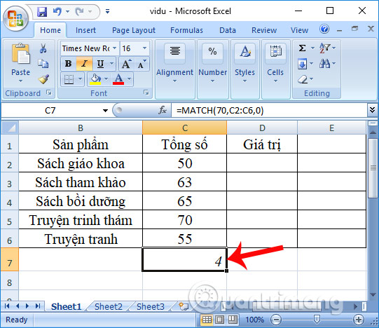
Look for the location of value 70 in the data table. We will have the input formula =MATCH(70,C2:C6,0) and then press Enter.

Match function in Excel: How to use the Match function with examples Picture 15

The returned result will be the position of value 70 in the Total column as the 4th position.

Match function in Excel: How to use the Match function with examples Picture 16

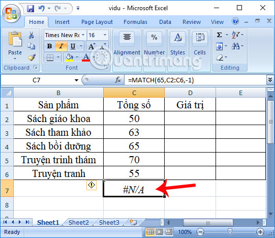
Case 3: Search type is -1

We will have the formula =MATCH(65,C2:C6,-1) as shown below.

Match function in Excel: How to use the Match function with examples Picture 17

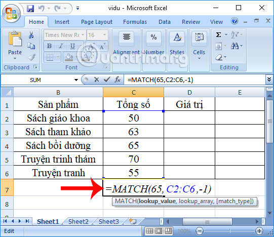
However, because the array is not sorted in descending order, an error will be reported as shown below.

Match function in Excel: How to use the Match function with examples Picture 18

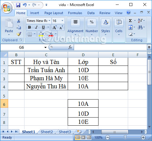
Example 2:

Given the student group data table below. Find the student's class order in this data table, with the order given below.

Match function in Excel: How to use the Match function with examples Picture 19

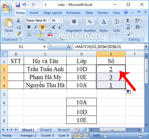
The order search formula is =MATCH(D2,$D$6:$D$8,0) then press Enter.

Match function in Excel: How to use the Match function with examples Picture 20

Immediately after that, the returned results will be the exact order of students by class, arranged according to the given rules.

Match function in Excel: How to use the Match function with examples Picture 21

In summary, things you need to remember when using the Match function in Excel:

1. Purpose: Determine the position of any item in an array.
2. Return value: A number representing a position in lookup_array.
3. Argument:
   1. Lookup_value: Lookup value in the array.
   2. Lookup_array: Cell range or array reference.
   3. Match_type - [optional] 1 = (default) next exact or smallest value, 0 = exact match, -1 = next largest or exact value.
4. Formula: =MATCH(lookup_value, lookup_array, [match_type])

Above is everything you need to know about the MATCH function in Excel. Even though it's just a function to find values, not calculate values, it is extremely useful when you need to arrange data reasonably and logically.

Basically, using the Match function in Microsoft Excel is not too difficult if you understand all the basic information above. Besides the Match function, Excel has many other useful functions. Let's continue to learn about Excel functions with QuanTriMang in the following articles!

Wishing you success!

Jessica Tanner

Update 10 July 2024