The LEFT function: Extracts characters from the left side of a string in Excel.

What is the Left function in Excel ? How to use the Left function in Excel ? Let's find out together with TipsMake.com!

 

Microsoft Excel is renowned as spreadsheet software capable of handling large volumes of data. You can input a large amount of data and then use intelligent Excel functions to automatically calculate the results. In this article, we will explore the LEFT function – one of Excel's commonly used text functions.

The LEFT function belongs to the string manipulation function group and is used to extract characters from the left side of a text string. The LEFT function is often used for quick information retrieval, instead of manually searching for information or character strings. In particular, the LEFT function can be combined with other lookup functions in Excel to handle complex data tables, such as combining the LEFT function with the Vlookup function . This article will guide you on how to use the LEFT function in Excel.

1. How to use the Vlookup function in Excel
2. How to combine the Sumif and Vlookup functions in Excel
3. Use the VLOOKUP function to merge two Excel spreadsheets.
4. The COUNTA function: How to use the function to count cells containing data in Excel.

 

The LEFT function formula in Excel

The LEFT function has the syntax =LEFT(text;[num_chars]) . Where:

1. Text is a required text string; it is either a text string or a cell reference to a text string containing the characters you want to extract.
2. Num_chars is an optional argument; it specifies the number of characters you want the LEFT function to search for, starting from the leftmost position in the text.
3. Num_chars must be greater than or equal to zero; if num_chars < 0, the function will return the #VALUE! error.
4. If Num_chars is greater than the length of the text, the LEFT function will return the entire text.
5. If num_chars is omitted, the default value of num_chars is 1.

Notes on using the LEFT function in Excel

1. The LEFT function in Excel should be used to extract characters starting from the left side of the text.
2. Number_of_characters is optional and defaults to 1.
3. LEFT in Excel will also extract the digits (0-9) from numbers.
4. Numerical formatting (i.e., the currency symbol $) is not part of the number. Therefore, it is not calculated or extracted by the LEFT function.

How do I open the LEFT function in Excel?

1. Simply enter the desired LEFT formula in Excel into the required cell to obtain the desired return value on the argument.

2. You can manually open the LEFT formula in the Excel dialog box within the spreadsheet and enter the text and number of characters.

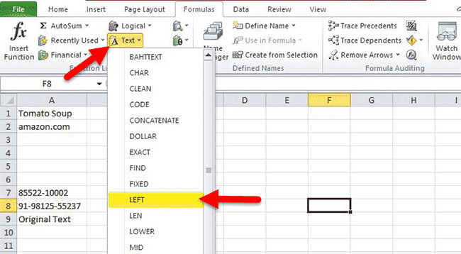
3. From the spreadsheet above, you can see the LEFT function formula option in Excel under the Text tab in the Formulas section of the menu bar.

4. To open a LEFT formula in the Excel dialog box, click the Text tab in Formulas and select LEFT. See the example below.

 

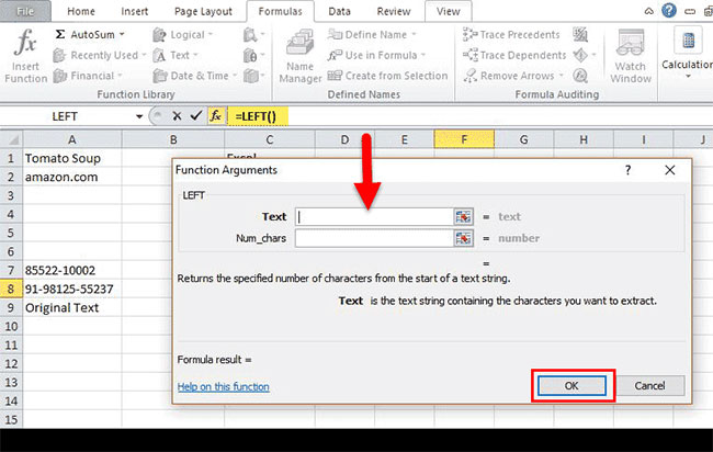
5. The dialog box above will open where you can enter the arguments to achieve the formula result.

Some formulas for the LEFT function in Excel.

Extract a substring before a given character.

You can use the general formula below to get a substring that precedes any other character:

The LEFT formula above in Excel is used when you want to extract a portion of a text string that precedes a specific character. For example, if you want to extract names from a column of full names or you want to extract the country code from a list of phone numbers.

Remove the last N characters from a string:

You can use the following general formula to remove the last N characters from a string.

The LEFT formula above in Excel is used when you want to remove certain characters from the end of a string and move the rest of the string to another cell. The operation of the LEFT formula in Excel is based on the following logic: The LEN function is used to get the total number of characters in a string. This LEFT formula in Excel excludes unwanted characters from the total length and returns the remaining characters.

Instructions on using the LEFT function in Excel

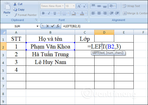
Example 1: Using the LEFT function to find a character

In the table below, use the LEFT function to find the first 3 characters in cell B2. Enter the formula =LEFT(B2,3) and press Enter.

 

As a result, we get 3 characters from left to right of the string in cell B2.

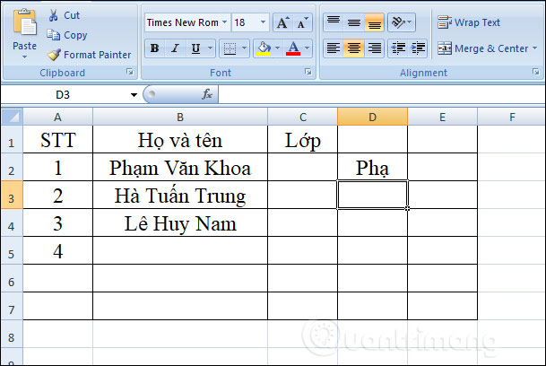
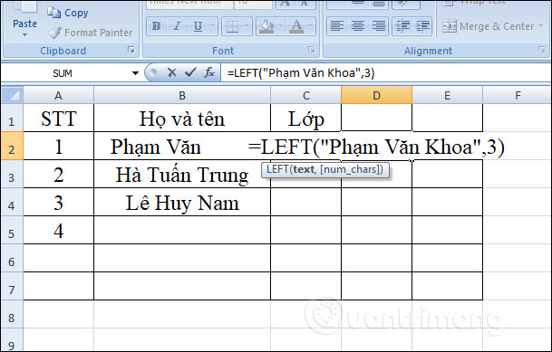
Alternatively, in the input formula, you can replace the cell containing the string with a character enclosed in quotation marks, as shown in the image.

Example 2: The LEFT function combined with the SEARCH function

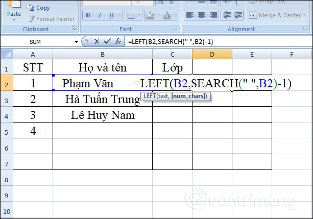
When combining these two functions, we can use them to search for the string preceding a specific character, for example, extracting the last name from the full name column, or extracting the country code minus the phone number. Since the full name column is separated by spaces, we use the formula =LEFT(B2,SEARCH(" ",B2)-1) and press Enter.

Then -1 is used to avoid extracting space characters during character search.

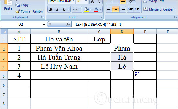
The result is that you get the last name string in the cell. Drag down to the cells below to see other results.

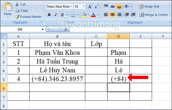
For the phone number you want to extract the country code for, after the dot, enter the formula =LEFT(B5,SEARCH(".,"B5)-1) and press Enter.

 

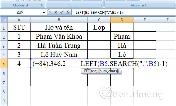
The result will only extract the country code from the phone number.

Example 3: Combining the LEFT function with the LEN function

The LEN function is often used in combination with string retrieval functions. When combined with the LEFT function, the LEN function is used to remove specific characters from the end of a string. The combined formula is =LEFT(text,LEN(text)-characters to remove).

The LEN function takes the total number of characters in a string, then subtracts the number of characters to be removed from the total length of the string. The LEFT function will return the number of remaining characters.

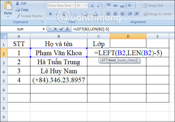
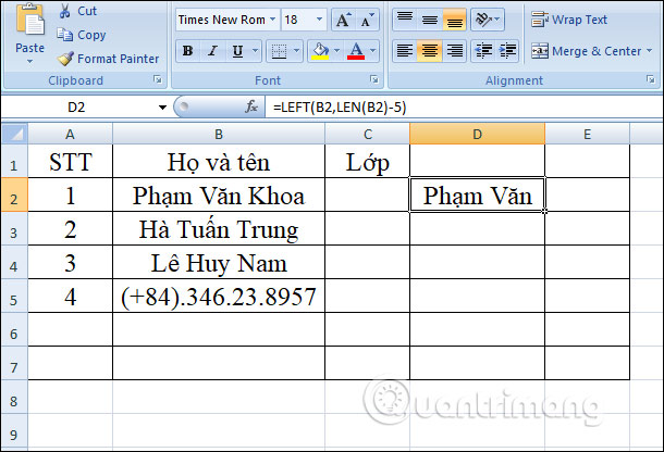
For example, to remove 5 characters from the string in cell B2, enter the formula =LEFT(B2, LEN(B2)-5) and press Enter.

The result is the remaining string of characters after removing the last 5 characters, including the space.

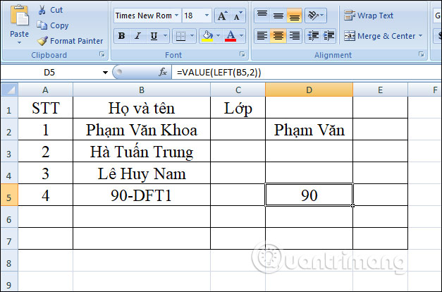
Example 4: Combining the LEFT and VALUE functions

When these two functions are combined, they return numeric characters instead of text strings, unlike when using the LEFT function alone. For example, to output the first two characters of the string in cell B5, enter the formula =VALUE(LEFT(B2,2)).

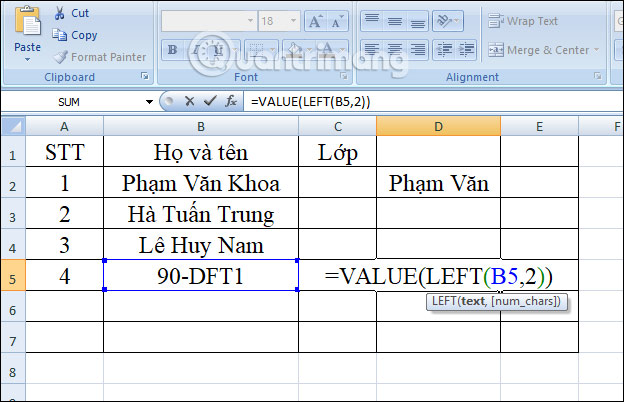
The result is the number we are looking for, as shown in the image.

The LEFT function in Excel is not working - causes and solutions.

If Excel's LEFT function isn't working correctly in your spreadsheet, it's most likely due to one of the following reasons.

1. The Num_chars argument is less than 0.

If your Excel LEFT formula returns a #VALUE! error , the first thing to check is the value in the num_chars argument. If it's a negative number, simply remove the minus sign to fix the error (of course, it's highly unlikely someone would intentionally put a negative number there, but human mistakes are quite common).

 

Typically, a VALUE error occurs when the num_chars argument is represented by a different function. In this case, copy the function to another cell or select the function in the formula bar and press F9 to see what value it corresponds to. If the value is less than 0, then check for function errors.

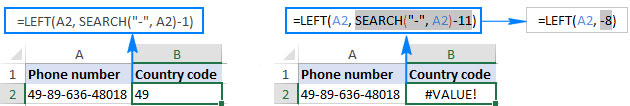
To illustrate this point more clearly, let's use the LEFT formula used to extract the country code: LEFT(A2, SEARCH("-", A2)-1) . As you may recall, the SEARCH function in the num_chars argument calculates the position of the first hyphen in the original string, from which we subtract 1 to remove the hyphen from the final result. If you accidentally replace -1, for example, with -11, the formula will throw a #VALUE error because the num_chars argument is equivalent to a negative number: The formula on the left doesn't work because the num_chars argument is less than 0 .

2. Line spacing in the original text

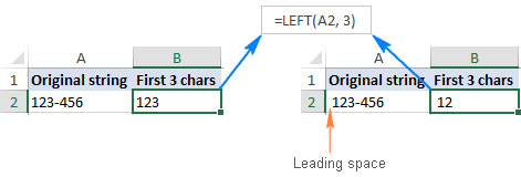
If your Excel LEFT formula fails for no apparent reason, check the original values ​​for leading spaces. If you copied your data from the web or exported it from another external source, many such spaces may be present before text entries without you realizing it, and you'll never know they're there until a problem occurs. The following image illustrates an Excel LEFT function malfunctioning due to leading spaces in the original string.

To remove leading spaces from your spreadsheet, use Excel's TRIM function or the Text Toolkit add-in .

3. Excel LEFT does not work with dates.

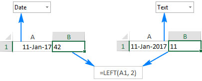
If you try to use Excel's LEFT function to extract individual parts of a date (such as the day, month, or year), in most cases you'll only get the first few digits of the number representing that date. The problem is that in Microsoft Excel, all dates are stored as integers representing the number of days since January 1, 1900, which is stored as the number 1. What you see in a cell is just a visual representation of the date, and how it's displayed can easily be changed by applying a different date format.

For example, if you have January 11, 2017 in cell A1 and you try to extract the date using the formula LEFT(A1,2), the result will be 42, which are the first two digits of the number 42746, representing January 11, 2017 in the Excel system.

To extract a specific part of a day, use one of the following functions: DAY, MONTH, or YEAR.

If your date is entered as a text string, the LEFT function will work without any problems, as shown in the right-hand part of the screenshot: Excel LEFT does not work with dates but works with text strings representing dates.

4. Missing currency symbol

If the original text has currency or accounting formatting applied, this symbol is not part of the characters in the cell. This symbol only appears when it is accompanied by specific number formatting. The LEFT function is a text function. Therefore, it will convert all values ​​to text format.

A helpful solution here is to combine LEFT with the VALUE function to convert text into a number. Then you can choose your desired number format.

5. The LEFT function returns fewer characters than expected.

If you know the number of characters that make up the desired output but the LEFT function formula only returns a certain number of characters, you may need to add more spaces to the original text.

Instead of deleting them manually, you can use the TRIM function to remove them.

=LEFT(TRIM(A2),7)

Some things to remember when using the LEFT function in Excel.

1. An error #VALUEoccurs if the argument [num_chars] is less than 0.
2. Dates are categorized as numbers in Excel, and only cell formatting makes them appear as dates in the spreadsheet. Therefore, if you want to use the LEFT function for dates, it will return the first few characters of the number representing the date.

For example, 01/01/1980 represents the number 29221. Therefore, applying the LEFT function to a cell containing the date 01/01/1980 (and requesting 3 characters) will give you the result 292. If you want to use LEFT on dates, you can combine it with the DAY, DATE, MONTH, or YEAR functions. Alternatively, you can convert date cells to text using Excel's Text-to-Column tool.

The above explains how to use the LEFT function to extract characters from the left side of a string, along with examples of combining the LEFT function with other functions. If an error occurs, the user should check num_charsif the value is greater than 0.

Good luck with your project!