How to Wrap Text in Excel 2007, 2010, 2013, 2016

This guide explains how to wrap Text in Excel 2007, 2010, 2013, 2016, with clear steps, practical tips, and important checks before you begin.

Method 1: Use the key combination Alt + Enter

When you want to make a new line in a cell, at any position in the cell, you use this method to create a new line.

Step 1: First, you put the cursor in the position you want to line down the cell.

If you are entering data, then stop where you want the line to go.

Step 2: After you've determined the position of the line you click the Alt + Enter combination to enter the line, this time from the position you put the mouse cursor will be down the line immediately, you just need to align content accordingly.

And if you are entering the data that you line down, the mouse cursor will be down the line, you continue to enter the data you want.

Method 2: Use the Wrap Text feature

The Wrap Text feature in Excel helps you automatically wrap text in a cell, you do not need to choose the starting position of the line, but Excel will automatically wrap the line depending on the width of the cell. The content will be in a new line until all the data in the cell is displayed.

Step 1: Select the cell that you want to auto-wrap, you can select multiple cells by holding Ctrl and use your mouse to select the cells you want to go down the line, cells that can contain data or blank cells.

;

Step 2 : Select Home -> Wrap Text to select the automatic newline feature.

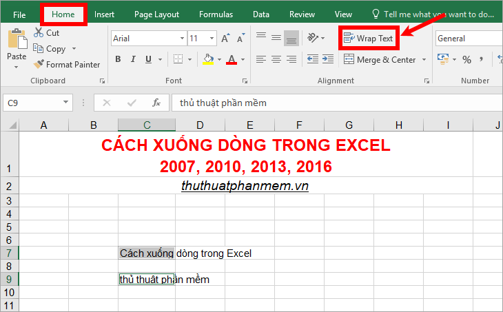
Immediately the cells you select will be automatically added, the position down the line depending on the width of the cells and the number of lines according to the length of the data in the cell.

You just need to align the data cell, if you want the data to line with the content, you can adjust the width of the cell.

With white cells, when you use Wrap Text to create a new line, when you look at it, you will see that the cells will not change, but when you enter the data, the width of the cell will be automatically adjusted when the mouse enters the width of the cell. Move to the bottom of the line.

Method 3: Auto-break associated with cell data alignment.

This method is an extension of Option 2, you can use Wrap Text in Format Cells to both line and align the data according to what you set. You do the following:

Step 1: Select one or more cells need to go down the line automatically, then right-click and select Format Cells or Ctrl + 1 key combination to open the Format Cells dialog box .

Step 2 : In the Format Cells dialog box , select the Alignment tab. Here in the Text alignment you can choose the alignment of the text in the box: Horizontal (horizontal); Vertical (vertical). In the Text control section, tick the box before Wrap text to select the automatic newline feature.

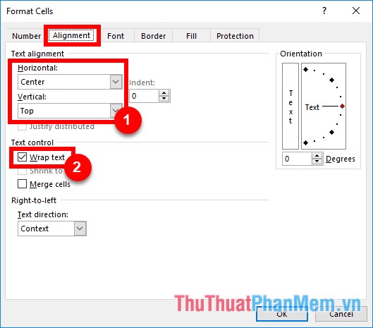
You can set other customizations in the Font, Border, Fill tab of the Format Cells dialog box, after the setup is complete, select OK .

That way, the cells you select will be automatically downlined and aligned to the customizations you have set.

The above is the way down the line in Excel 2016, with versions of Excel lower than 2007, 2010, 2013 you also apply the same. Good luck!