How to use the LOOKUP function in Excel - Data search function

The LOOKUP function in Excel has many uses. This article will show you how to use the LOOKUP function in Excel simply and quickly.

 

Searching in a Microsoft Excel spreadsheet is fairly easy using the keyboard shortcut Ctrl + F. However, you can use more sophisticated tools to find and extract data based on specific values.

Microsoft Excel provides many functions to help you do this easily, and LOOKUP is just one of them.

What is the LOOKUP function in Microsoft Excel?

The LOOKUP function in Excel references a cell to match a value in another row or column based on that cell, giving the user a corresponding result.

Some common ways to use the LOOKUP function:

1. Find the exact or approximate value.
2. Data can be searched both vertically and horizontally.
3. Easier to use and no need to select the entire table.

Concepts you need to know in the LOOKUP function formula

1. Lookup - To find a specific value in a data table.
2. Lookup Value - A search value
3. Return Value - The value in the same location but a different row or column, depending on whether you want to look up the data horizontally or vertically.
4. Master Table - The table where you receive the appropriate value.

The Lookup function can be used in two forms: vector and array. Each form has a different formula and application scenario. This article will guide you on how to use the Lookup function in Excel.

1. How to use the Vlookup function in Excel
2. How to use the Hlookup function in Excel
3. How to combine the Sumif and Vlookup functions in Excel

Instructions on using the Lookup function in Excel

The vector lookup function is used to find a value within a range of one row or one column, and return the value from the same position within a second range of one row or one column. This vector lookup is useful when you want to define the range containing the values ​​you want to compare, or when the search range contains multiple values ​​or values ​​that may change.

 

Array search is used to find a specified value in the first column or row of an array, and then return the value from the same position in the last column or row of the array. Array search is used when the search range has few values, the values ​​remain unchanged, and they must be sorted.

1. Use the Lookup function as a vector.

The formula is =Lookup(Value to search for,Range containing the value to search for,Range containing the result value) .

The value to be searched for can be a number, text, logical value, name, or a reference to a value.

The search area contains text, numbers, or logical values. The values ​​within this area must be sorted in ascending order to avoid errors.

The range containing the result value can be a single row or a single column.

Note:

1. If the desired value is not found, the smallest value within the range containing the desired value will be used.
2. If the value to be found is smaller than the smallest value in the range containing the value to be found, the error #N/A will be displayed.

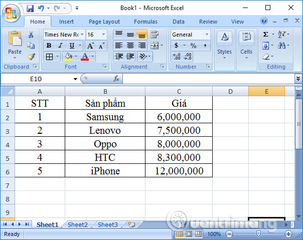
We will apply this to the table below. For example, if you want to buy a phone in the price range of 7,500,000 VND, what type of phone would you look for? And if you want to find a phone in the price range of 13 million VND, what type would you look for?

Step 1:

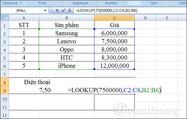
In the result input field for phones with a range of 7,500,000 users, enter the formula =LOOKUP(7500000,C2:C6,B2:B6) and press Enter. If using numbers, do not use delimiters between the units digits.

 

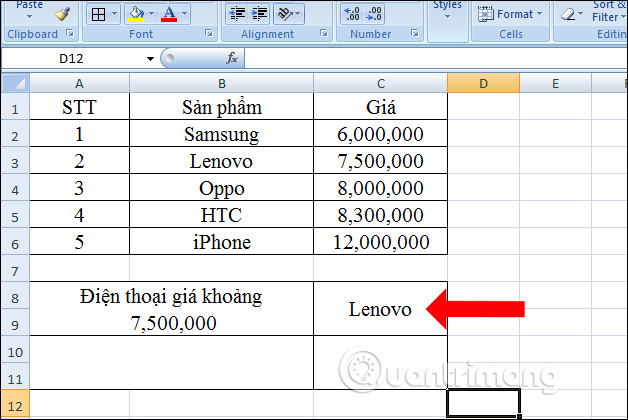
The result will show the phone model as Lenovo.

Step 2:

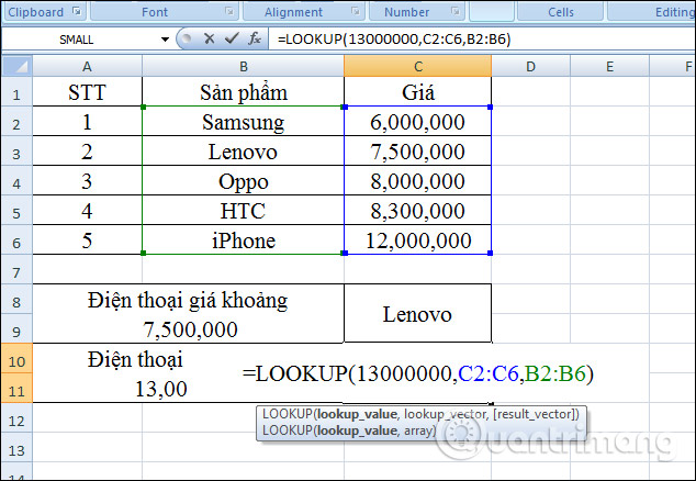
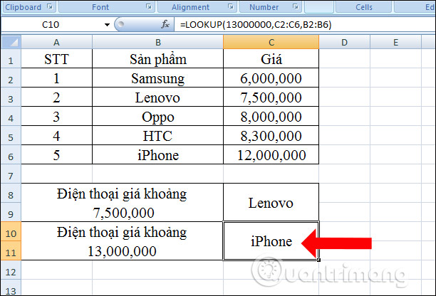
To find phone models within the range of 13 million, we enter the formula =LOOKUP(13000000,C2:C6,B2:B6) into the result cell and then press Enter.

The value 13,000,000 is not within the data range, so the Lookup function will search for a value less than 13,000,000.

As a result, we will have a list of recommended iPhone models to buy within the price range of 13 million VND.

 

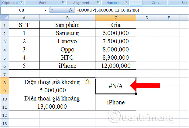
If you need to find a phone in the 5 million VND price range, you will get a #N/A error as shown below. This is because the value 5,000,000 is less than the minimum value in the table, which is 6,000,000. The search result will only show a price range between 6,000,000 and 12,000,000 VND.

2. Use the Lookup function as an array.

The syntax is =LOOKUP(Value to search, Search range) .

The value to be found is the value that the Lookup function needs to search for within an array.

The search area is the range of cells containing the text, numbers, or logical values ​​that you want to find.

Note:

1. If the desired value is not found, the nearest smaller value within the search range will be used.
2. If the value to be found is smaller than the smallest value in the first row or column, the Lookup function will return the #N/A error.
3. If the array has more columns than rows, the Lookup function will search for the desired value in the first column.
4. The values ​​in the search area must be sorted in ascending order.

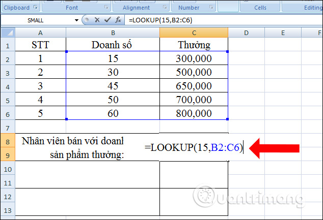
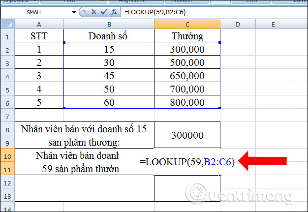
We will process the data table below with sales achieved and bonuses for sales milestones achieved. Calculate bonuses for employees who sold 15 products and for employees who sold 59 and 65 products, respectively.

Step 1:

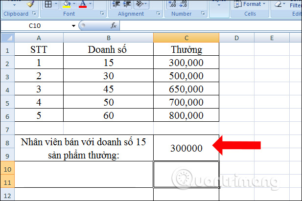
In the cell showing the bonus result for the employee who sold 15 products, enter the formula =LOOKUP(15,B2:C6) .

The reward results will be as shown below.

Step 2:

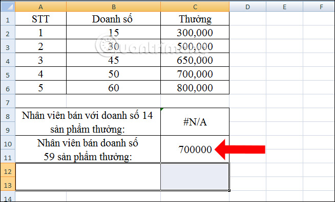
Continuing in the result cell for the bonus for the employee who sold 59 products, you enter the formula =LOOKUP(59,B2:C6) .

 

The bonus for an employee who sells 59 products will still be 600,000. Although the number 59 is not in the table, it will still have value.

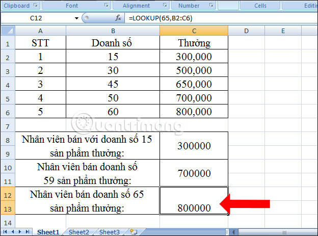
Step 3:

In the result box, the reward for the product is 65. We enter the formula =LOOKUP(65,B2:C6) and press Enter, and the result will be 800,000 as shown in the image.

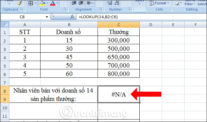
If a user searches for a reward for someone who has purchased 14 products, an error will be displayed because the value being searched for is smaller than the smallest value in the table.

Things to note when using the LOOKUP function in Excel

Use the LOOKUP function to look up a value in a column or row range, and retrieve the same value from a different column or row range. The LOOKUP function comes in two forms: vector and array.

The LOOKUP function accepts three arguments: lookup_value, lookup_vector, and result_vector. The first argument, lookup_value, is the value to search for. The second argument, lookup_vector, is a row or column to search. LOOKUP assumes lookup_vector is sorted in ascending order. The third argument, result_vector, is a result row or column. Result_vector is optional.

When result_vector is provided, LOOKUP identifies a match in lookup_vector and returns the corresponding value from result_vector. If result_vector is not provided, LOOKUP returns the matching value found in lookup_vector.

LOOKUP has an efficient way of handling specific problems, especially in data retrieval. Therefore, you can rest assured when using it.

See more:

1. How to use the Concatenate function in Excel
2. How to use the SUMPRODUCT function in Excel
3. How to use the AVERAGEIF function in Excel

Good luck with your project!