3 Excel functions to help build lookup formulas extremely quickly

Slow lookup formulas can be a productivity killer when working with large data sets. To address this issue, this article examines Microsoft Excel 's optimized lookup functions and how to combine them to build blazing fast formulas that can handle even large spreadsheets with ease.

3. Combining LET and XLOOKUP

Eliminate repetitive calculations

Formulas can sometimes become long and complicated, especially when you need to perform the same calculation multiple times in a formula. This not only makes the formula difficult to read, but also reduces performance, as Excel has to calculate the same result multiple times.

The solution to this problem is the LET function , which allows you to declare variables directly inside the formula. You calculate it once, give it a name, and then just use that name whenever you need the result. The syntax is simple:

=LET(name1, name_value1, [name2, name_value2], calculation)

1. name1 : The name for your first calculation (e.g. "rating").
2. name_value1 : The calculation itself (e.g. an XLOOKUP formula).
3. calculation : The final formula uses the name you just defined.

Let's say you have a task that requires assigning a status based on an employee's current rank. If their rank (found by employee ID) is five, they'll be placed in the "Top Tier" group. If their rank is one, they'll be placed in the "On Watchlist" group. Otherwise, they'll be placed in the "Standard" group.

Without LET, you would have to write the XLOOKUP function twice, like this:

=IF(XLOOKUP(A2, A:A, AC:AC)=5, "Top Tier", IF(XLOOKUP(A2, A:A, AC:AC)=1, "On Watchlist", "Standard"))

But when using LET, the formula becomes much cleaner. You only have to calculate XLOOKUP once and assign it to the name "rating".

=LET(rating, XLOOKUP(A2, A:A, AC:AC), IF(rating=5, "Top Tier", IF(rating=1, "On Watchlist", "Standard")))

This formula looks up the employee ID from cell A2 in column A , gets their numerical rating from column AC , and then sorts the performance.

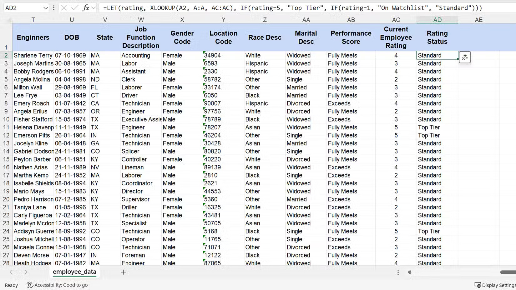
The LET function caches the rank lookup once, preventing Excel from repeating the same XLOOKUP calculation in nested IF statements. This formula is significantly easier to read and debug.

2. INDEX and MATCH work great together

They generate the fastest lookup combinations

Before XLOOKUP came along, INDEX and MATCH were the only options for building quick lookups. Even now, this combination often outperforms newer functions in speed. On spreadsheets with tens of thousands of rows, this combination is significantly faster because it only processes the specific columns you reference, not the entire table.

Neither function does a complete lookup on its own. The MATCH function has one advantage: It finds the relative position (row number) of a value in one column. The INDEX function then takes that number and gets the corresponding value from another column.

First, let's look at the MATCH syntax. It tells you where your data is located.

=MATCH(lookup_value, lookup_array, [match_type])

1. lookup_value : The value you want to find.
2. lookup_array : The single column or row to search.
3. [match_type] : Use 0 for exact match, this is the value you will need in 99% of cases.

Next is the INDEX syntax, which will retrieve the result you want based on the position provided by the MATCH function.

=INDEX(array, row_num, [column_num])

1. array : The range of cells or array to retrieve values from.
2. row_num : Row number to retrieve value.

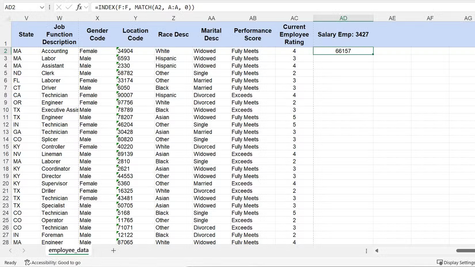
Let's say you need to find the salary range for employee ID 3,427. Use the following formula:

=INDEX(F:F, MATCH(A2, A:A, 0))

In this example, the MATCH part will first find the row number of the employee ID in cell A2 . The INDEX function will then take that number and return the value from that same row in the salary field column (column F). This is a compact and efficient method.

1. FILTER is the optimal lookup function

Replace multiple lookups at once

Standard lookups, including XLOOKUP, have a fundamental limitation — they stop and return the first match they find. But what if you need a list of all matching records? In versions of Excel prior to 2021, this required complex array formulas. Now, use the FILTER function instead. It extracts every record that meets your criteria.

If you've never used Excel's FILTER function, you're really missing out. It returns an array of values that automatically spill into the cells below the formula. This means you no longer have to guess how many results you'll get. The function automatically handles the output size for you, which is a huge time saver.

Here is the syntax of the FILTER function:

=FILTER(array, include, [if_empty])

1. array : This is the entire range of data you want the results from. This can be one column or multiple columns.
2. include : This is your logical test. It's a range of cells followed by a condition, such as checking if the value in a column equals "Active".
3. [if_empty] : An optional argument for what to display if no results are found.

Let's say a manager, Peter O'Neill, wants a list of all his employees. You need to get the full name, start date, and salary of each employee listed on the supervisor list. With FILTER, you can get this entire list with just one formula instead of having to do multiple separate lookups.

Here is the formula to get the job done:

=FILTER(D:F, I:I="Peter Oneill", "No Employees Found")

This formula tells Excel to return data from columns D through F for each row where the value in column I is "Peter O'Neill".

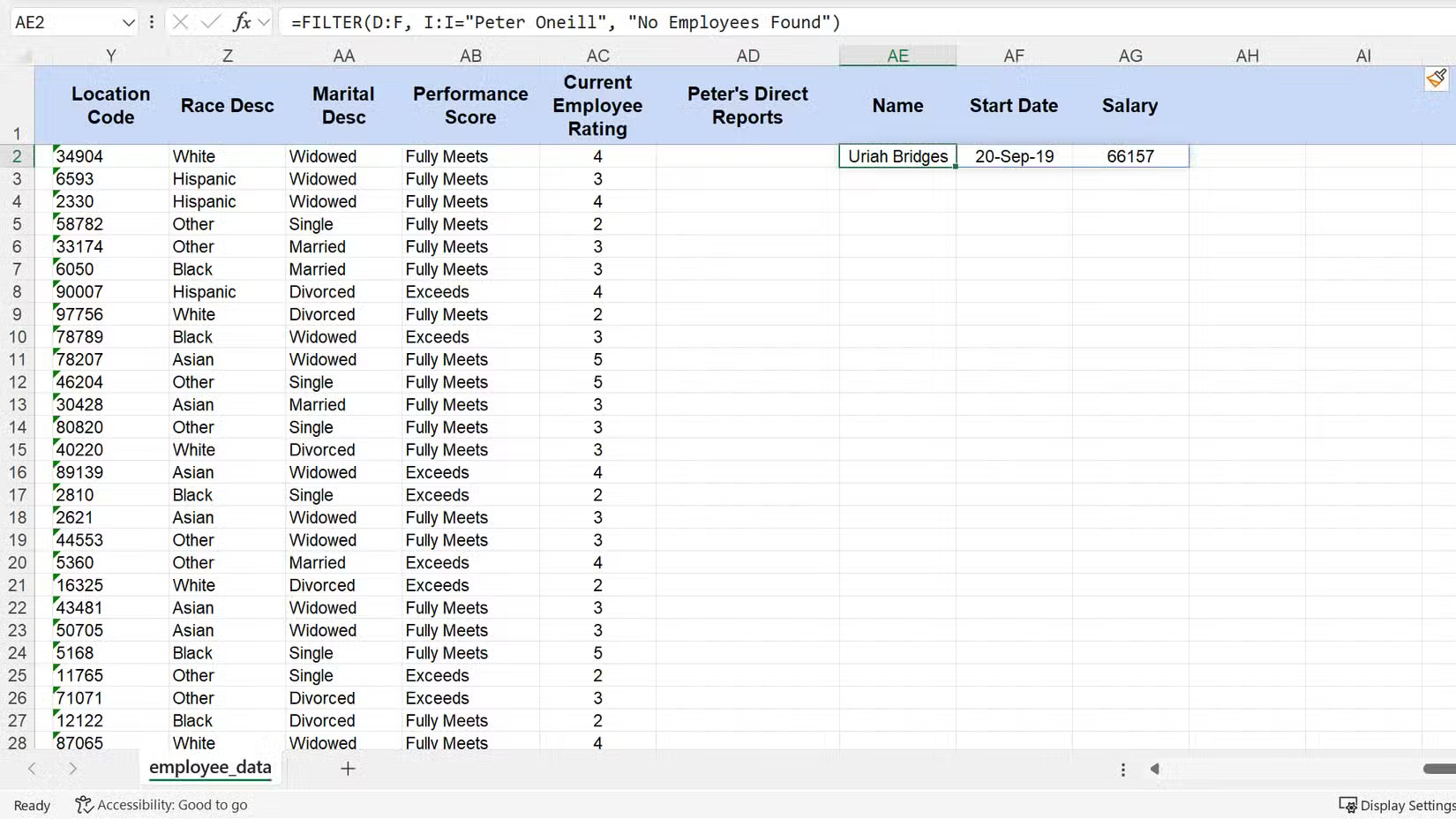
The results will automatically fill in the cells below, creating a neat, dynamic table. Thanks to this dynamic feature, this Excel trick will completely put an end to the annoyance of having to resize tables.

These methods cover every lookup situation you might encounter. XLOOKUP is the modern replacement for VLOOKUP. Use LET combinations for optimization, INDEX/MATCH for speed, and FILTER for multiple lookups.

Isabella Humphrey

Update 17 August 2025