How to use Lookup function in Excel

In Excel basic functions, Lookup function is often used by many people. Lookup is a reference function, a search function in Excel. This function will be used when you need to see a row or a column, looking for a value in the same position or column.

Lookup function will be used in two forms, vector and array. Each form will have a formula as well as a different application case. The following article will guide you how to use the Lookup function in Excel.

1. How to use Vlookup function in Excel
2. How to use Hlookup function on Excel
3. How to combine Sumif and Vlookup functions in Excel

Instructions for using Lookup function on Excel

The Vector form Lookup function is used to find a value in a range of 1 row or 1 column, and returns the value from the same position in the second range of 1 row or 1 column. This vector form will be used when you want to determine the range that contains the values ​​you want to compare, or when the range to be searched for is a range of values ​​or values ​​can be changed.

Array form to look up the value specified in the first column or row of the array, then return the value from the same position in the last column or row of the array. Array form used when the search range is low, the value remains the same and must be sorted.

1. Use the Lookup function in the Vector format

The formula is = Lookup (The value to look for, The area to find the value to look for, The container of the result value) .

The value to look for can be a number, a text, a logical value, a name, or a reference to a value.

The area to be searched for is text, number or logic value. The values ​​in this area must be sorted in ascending order so that no errors will occur.

The area containing the result value can be 1 row or 1 column.

Note:

1. If the value to be searched for is not available, the smallest value in the Value range will be used.
2. If the value to be searched for is smaller than the minimum value in the Area to be searched, the error will be reported # N / A.

We will apply to the statistics table below. For example, if you want to buy a phone for about 7,500,000, what kind of phone will you find? And if you want to find a phone in about 13 million, look for one.

How to use Lookup function in Excel Picture 1

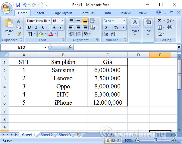
Step 1:

In the result input box for the phone in about 7,500,000 users enter the formula as = LOOKUP (7500000, C2: C6, B2: B6) and press Enter. If using numbers, do not use unit separators.

How to use Lookup function in Excel Picture 2

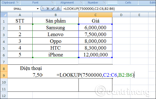
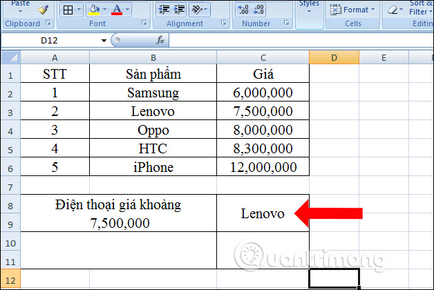
The result will be the Lenovo phone.

How to use Lookup function in Excel Picture 3

Step 2:

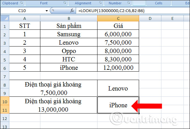
To find the phone line in about 13 million, enter the formula in the result box = LOOKUP (13000000, C2: C6, B2: B6) and press Enter.

The value of 13000000 is not in the data area, so Lookup will look for a value less than 13000000.

How to use Lookup function in Excel Picture 4

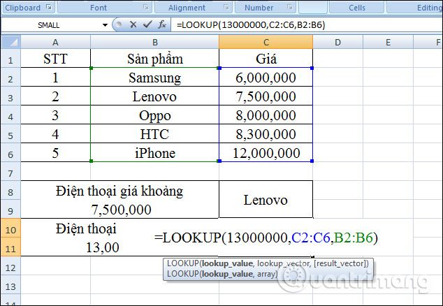
As a result we will have an iPhone phone company that should buy it for about 13 million.

How to use Lookup function in Excel Picture 5

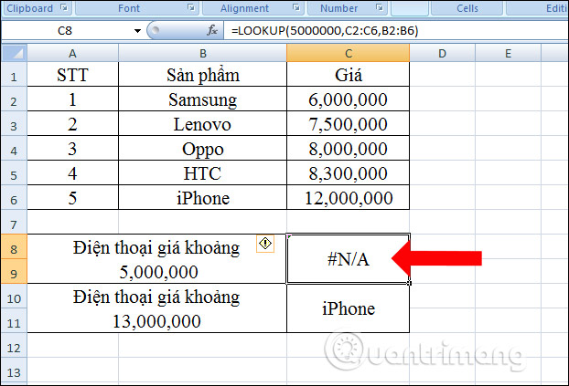
If you need to find a phone within 5 million VND, you will report # N / A error as shown below. So worth 5,000,000 less than the smallest value in the table is 6,000,000 and report an error. The result of the value you need to find will be in the range of 6,000,000 to 12,000,000 only.

How to use Lookup function in Excel Picture 6

2. Use the array Lookup function

The syntax is = LOOKUP (Search value, Search area) .

The value to look for is the Lookup function value to look for in an array.

The search area is the range of cells that contain text, numbers, and logical values ​​to look for.

Note:

1. If the value to be searched for is not found, the closest value in the Search Area will be taken.
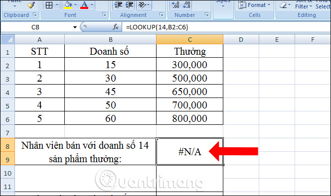
2. If the value to be searched for is smaller than the smallest value in the first row or column, Lookup will return the # N / A error.
3. If the array has more columns than rows, Lookup will search for the value to look for in the first column,
4. The values ​​in the Search Area must be sorted in ascending order.

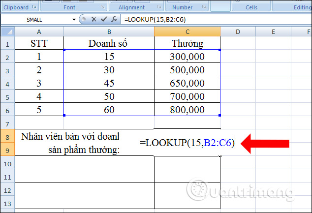
We will process the data table below with the sales achieved and reward the sales mark. Calculating bonus for employees selling 15 products and sales for employees is 59 products, 65 products.

Step 1:

In the results box for the 15 product sales staff, enter the formula = LOOKUP (15, B2: C6) .

How to use Lookup function in Excel Picture 7

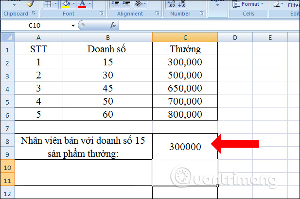
The reward results will look like the picture below.

How to use Lookup function in Excel Picture 8

Step 2:

Continue in the results box for employees to sell 59 products, enter the formula = LOOKUP (59, B2: C6) .

How to use Lookup function in Excel Picture 9

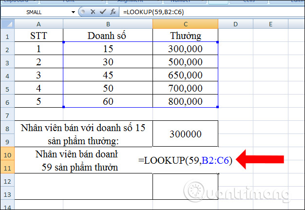
The reward results for employees reaching 59 products will still be 600,000. Although number 59 is not in the table, it will still have a return value.

How to use Lookup function in Excel Picture 10

Step 3:

In the reward box for the product is 65, we enter the formula = LOOKUP (65, B2: C6) and press Enter and the result will give 800,000 as shown.

How to use Lookup function in Excel Picture 11

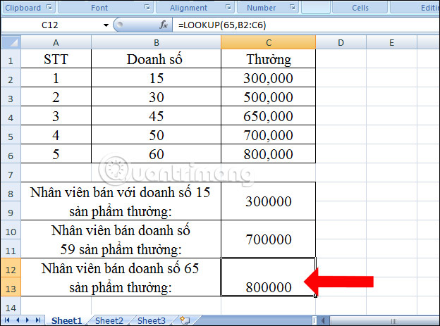
If a user finds a reward for a 14-person product, an error is reported, because the value to be searched is less than the smallest value in the table.

How to use Lookup function in Excel Picture 12

Here's how to use the detailed Lookup function in Excel. Lookup will be divided into two types, vector and array. The formula and usage of these two forms are not the same.

See more:

1. How to use ConcateNate function on Excel
2. How to use SUMPRODUCT function in Excel
3. How to use AVERAGEIF function in Excel

I wish you all success!