How to use Slicer to filter data quickly

What is a slicer in Google Sheets ? How to create a slicer in Google Sheets ? Let's find out together!

If you've ever worked with large datasets in Google Sheets, you know how difficult it can be to filter and analyze data. You can use filters, but applying and removing filters based on criteria is tedious. That's where slicers come in.

Slicers are interactive buttons that let you quickly filter data in Google Sheets without having to open the filter menu. You can create slicers for any column or row in your data and use them to show only values that match your criteria.

What is Slicer in Google Sheets? Why should you use Slicer in Google Sheets?

Slicers are similar to the filter tool in Google Sheets in that they can both filter data, but they do more than that. When you create a slicer, Google Sheets adds it as a button to your spreadsheet. This makes slicers more intuitive than traditional filters.

Slicers show you the headers available in your data, allowing you to select or deselect them with a simple click. You don't have to open the filter menu and scroll through a long list of options. Another great feature of slicers is that they display the entire chart. When you filter data through the slicer, the chart automatically updates to show the filtered data.

You can even change the appearance of the slicer by tweaking its size, font, or color. This way, the slicer won't be an odd addition to your spreadsheet. Instead, it will help you create a clean and efficient spreadsheet.

How to create slicers in Google Sheets

Create a slicer in Google Sheets in just a few clicks. You'll customize the slicer and change its settings after you create it. To create a slicer, go to the Data menu and click Add a slicer .

Once you do this, the slicer will appear in your spreadsheet. But that's not all. The slicer you just created will only work once you tell it what to slice. A slicer needs a range of data and column headers to work.

Using slicers with data tables

Slicers can instantly filter a data table without affecting other parts of the spreadsheet. Slicers don't remove cells, they just hide them, similar to the filter tool in Google Sheets.

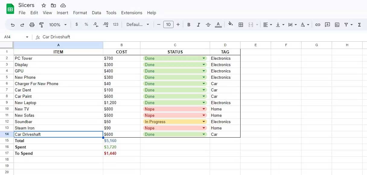
For example, consider the spreadsheet above. It is a long shopping list that includes the price, status, and category of each item. Let's say the goal here is to quickly filter the items by category (tag). Slicers are the easiest way to do this.

To use slicers in Google Sheets, you need a table with a header row like the table in the example above. Here's how you can filter data with slicers in Google Sheets:

1. Go to the Data menu and click Add a slicer .

2. Select the slicer and click the 3 vertical dots on the top right.

3. In the drop-down menu, select Edit slicer . This will open the slicer settings on the right.

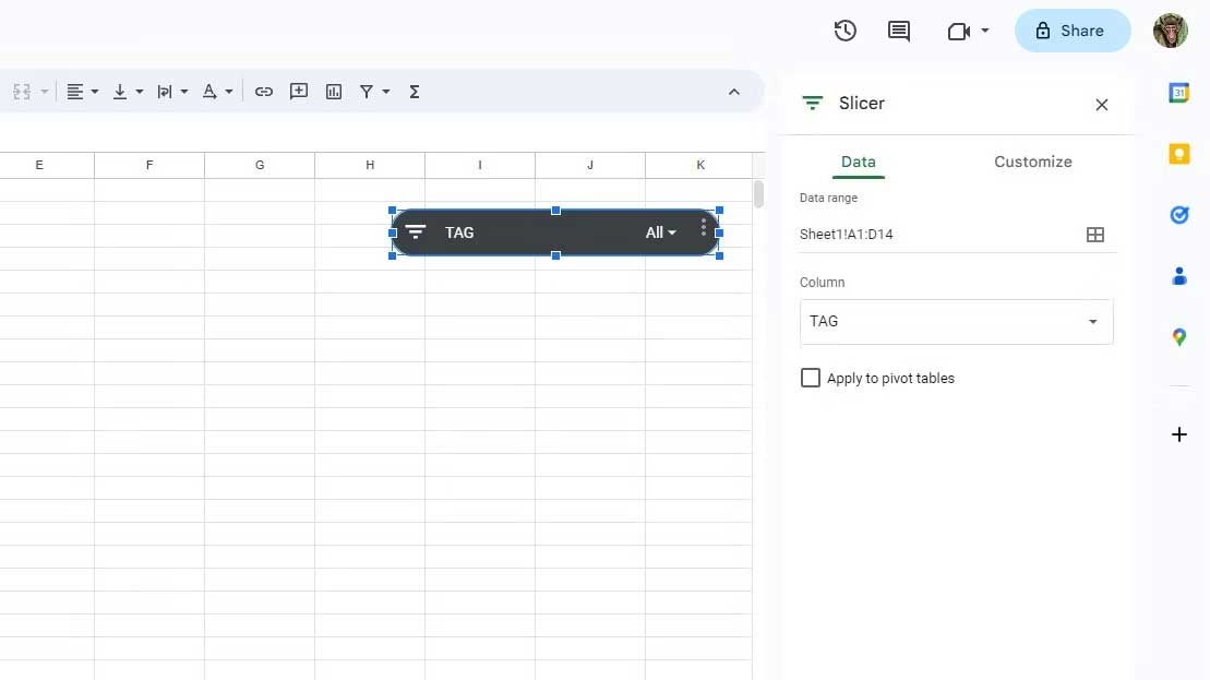
4. Enter data in Data range . That is A1:D14 in the example. Google Sheets will automatically read the column headers from this table.

5. Click the drop-down list in Column and select the column you want to filter data by. That's Tag in the example.

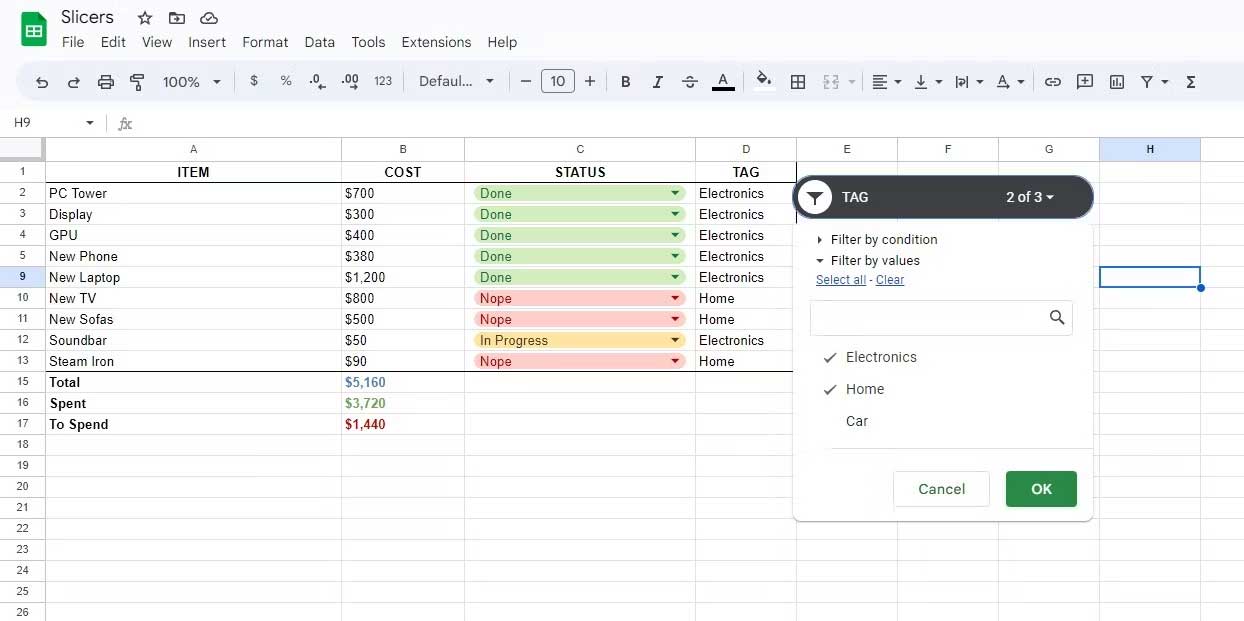
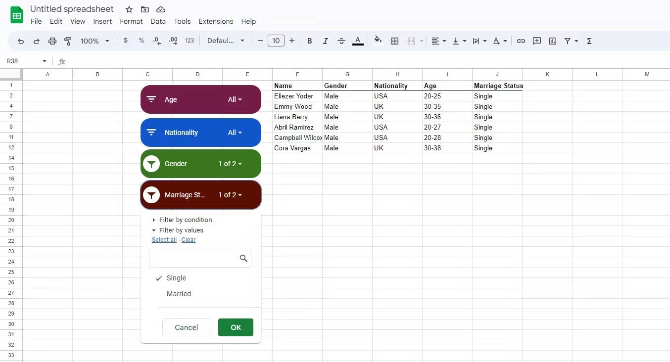
The slicer is now ready to use. Click the icon in the left corner of the slicer to open the filtering options. To select or deselect values in the slicer, click them, then click OK. The spreadsheet will change to show the desired results.

Note that cells not in the slicer data range (B15 to B17) remain unchanged.

Using Slicers with Charts

Another great way to use slicers in Google Sheets is to filter charts. This allows you to create dynamic charts that change based on your slicer selection.

You don't need to create a separate slicer for that chart. The slicer will filter both the data table and the chart based on the same data range like this:

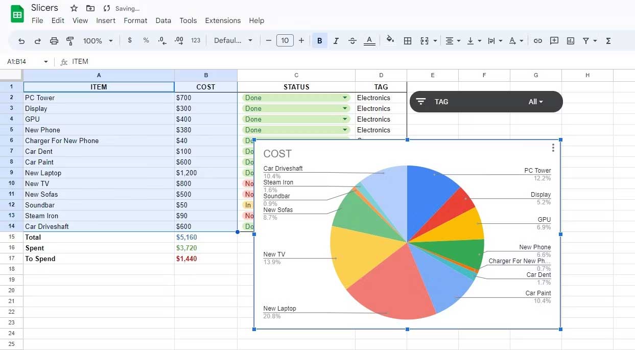
Each chart type in Google Sheets is suitable for a specific type of data. In this case, the best chart to illustrate the data in your spreadsheet is a pie chart.

1. Select the data you want to graph. For example, here is A1:B14 .
2. Go to the Insert menu > select Chart . Google Sheets should automatically detect and create a pie chart. If not, move on to the next step.
3. In the Chart editor , go to the Setup tab .
4. Change Chart type to Pie chart .

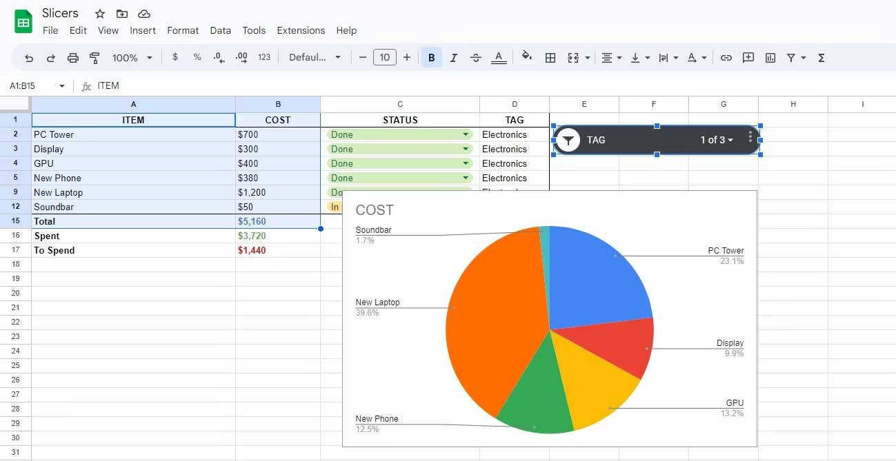
Now use the slicer and watch the pie chart change to illustrate the desired items. As you can see, you have just upgraded your chart from static to dynamic!

How to Edit Slicers in Google Sheets

You can edit a slicer in Google Sheets by changing its data settings, appearance, or location. Here are some things you can do:

1. To change the data range of the slicer filter, go to the Data tab in the slicer settings. You can select a different data range or change the filter criteria by changing the column.
2. To change the look of your slicer, go to the Customize tab in the slicer settings. You can change the look of your slicer by adjusting the title, title font, and background color.
3. To resize a slicer, select it and drag the blue dots around. There isn't much room to stretch the slicer's height, but you can stretch or shrink its width as you like.
4. To move a slicer, click it and drag it to a new location on the spreadsheet.

Above is how to use slicer in Google Sheets . Hope the article is useful to you.

Isabella Humphrey

Update 17 July 2025