Column order in Excel is reversed, why and how to handle it?

Is the column order in Excel reversed making you feel confused? Is this a problem and how to fix it? All these questions will be answered in detail by TipsMake.

Sometimes Excel will make you 'sweat' if you encounter a situation that you don't understand. In Excel, whether you have been practicing for a long time or are new to it, sometimes there are still some situations that you don't know how to handle. Reversed column order in Excel is also a case that confuses countless people. Don't worry, TipsMake has found a way to help you solve it.

Column order in Excel is reversed, why and how to handle it? Picture 1

Why is the column order in Excel reversed? How to handle?

Column order in Excel being reversed, or Excel having letters reversed is not an error. There is a high possibility that you have customized Excel incorrectly. Besides, there are some cases of reversing the order in Excel because users use tricks depending on their purposes. I will reveal both the fix and the reverse method for your reference.

Case in which Excel has the letters reversed

Regarding Excel's reversed text, it is highly likely that you have used the text rotation feature ( Orientation ) in Excel. Therefore, users can apply this feature to fix errors as follows:

In Excel that is being anagrammed > Click on the Home tab > Find the ab icon with the up arrow > Click on the arrow to open the list > Check to see which style the text in Excel is being rotated > Click on the style again That is the word that will return to the original.

Column order in Excel is reversed, why and how to handle it? Picture 2

Fix reversed Excel File

For example, columns A, B, C will normally display in order from left to right. But your Excel file is reversed and appears from right to left. It is highly likely that the user has enabled the 'Show sheet right-to-left' feature. To fix this situation, in the open and corrupted Excel file, click on the File > Options > Advanced tab in the list on the left.

Then, go to Default direction > Tick left-to-right > Click OK to save and you're done. 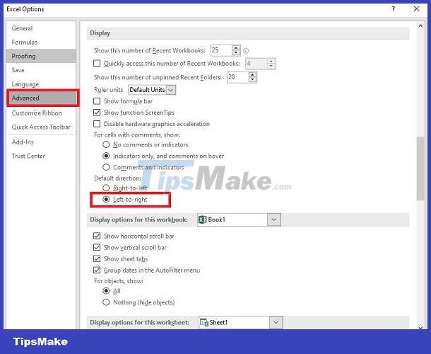Column order in Excel is reversed, why and how to handle it? Picture 4

Instructions on how to quickly reverse columns in Excel

Note: In Excel there is no built-in function to reverse or flip column order. Therefore, if you want to reverse data from bottom to top in Excel, reverse the column order, you need to perform different formulas and combinations of these formulas.

Currently, there are many ways for us to quickly reverse columns in Excel. Below are a few of the most popular and easy-to-implement methods.

1: Reverse data from bottom to top in Excel using helper columns

1. Step 1 : Create a column of data adjacent to the columns whose content you want to flip. The title of this column will be ' helper ' as shown.

Column order in Excel is reversed, why and how to handle it? Picture 5

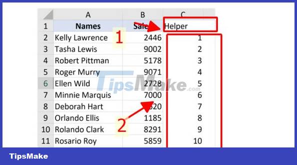
1. Step 2 : In the column you just created, enter the numbers from 1 to N one by one. N will be on the same line as the last data you want to reverse. You can do it quickly by entering numbers 1 and 2 respectively in the first 2 boxes. Then drag the mouse to automatically number!
2. B3 : Click to select all data including the data column you just created
3. B4 : Click on the data tab , then click on the ' sort ' icon
4. B5 : Click on ' helper ' in the sort by section.

Column order in Excel is reversed, why and how to handle it? Picture 7

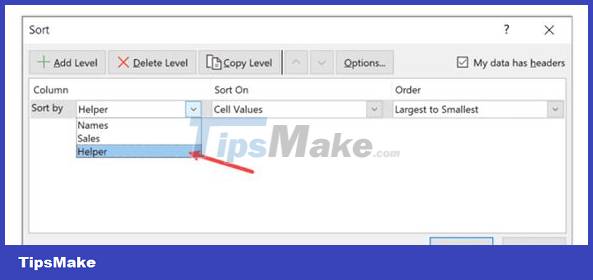
1. Step 6 : Continue clicking ' Largest to Smallest ' in the other section and finally click ' ok '

Column order in Excel is reversed, why and how to handle it? Picture 9

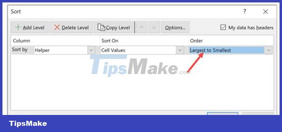
At this time, the data in the table will be reversed in order based on the change in the order of the helper column. After completing the data reversal. We just need to delete the helper column.

2: Use the reverse column function in Excel

We can also use the function to reverse columns in Excel. Here's how to use the index function to do this.

1. Step 1 : Click on a new location in the Excel table, this will be where the results will be displayed when you reverse the data. Then highlight the location where you intend to contain the data after inversion.
2. Step 2 : Enter =index then click to open parenthesis '('
3. Step 3 : Highlight the entire data area you want to reverse and press the F4 key on the keyboard.

Column order in Excel is reversed, why and how to handle it? Picture 11

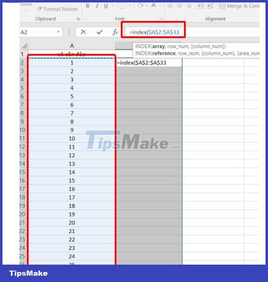
1. Step 4 : Enter the comma ' , ' then enter the rows function and press the opening parenthesis key ' ( '.

Column order in Excel is reversed, why and how to handle it? Picture 13

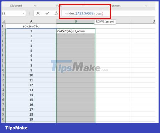
1. Step 5 : Black out the entire area you want to reverse data. Then click on the part behind the colon as shown and press the F4 key.
2. Step 6 : Press closing parenthesis ')' twice and press crtl + enter . Your content will now be quickly reversed.

Column order in Excel is reversed, why and how to handle it? Picture 15

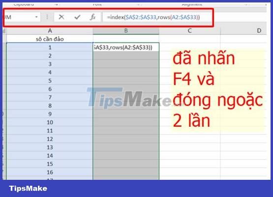
Above is detailed information about the column order in Excel being reversed. Hope my guide will be useful to you.

Samuel Daniel

Update 08 December 2023