IRR function in Excel - Usage and examples

In Excel financial functions, users cannot ignore IRR - the function that returns the internal rate of return for a series of cash flows. So how does the function structure and usage of the IRR function? Please read the article below.

What is the internal rate of return?

In corporate finance, the Internal Rate of Return (IRR) is a ratio of profits used in capital budgeting to measure and compare return on investment. More specifically, the discount rate at which the net present value of the investment (negative cash flow) is equal to the net present value of the investment (positive cash flow).

Internal rate of return is often used to assess the necessity of an investment or project. The higher the internal rate of return for a project, the more desirable it is to execute the project. Assuming all projects require the same amount of investment, the project with the highest IRR level will be considered best and executed first.

IRR calculation formula:

(NPV = sumlimits_ {t = 1} ^ n {frac {{{C_t}}} {{{{(1 + r)} ^ t}}}} - {C_0} = 0)

Inside:

1. t: is the time to calculate cash flow.
2. n: is the total time of project implementation.
3. r: is the discount rate (IRR).
4. ({{C_t}}): is the net cash flow at time t.
5. ({{C_0}}): is the initial cost to implement the project.

Specific example: If an investment project can be put in place by the sequence of cash flow.

Cash flow ({{C_n}})

0

-4000

first

1200

2

1410

3

1875

4

1050

The IRR is then given by the formula:

(NPV = - 4000 + frac {{1200}} {{{{(1 + r)} ^ 1}}} + frac {{1410}} {{{{(1 + r)} ^ 2}}} + frac {{1875}} {{{{(1 + r)} ^ 3}}} + frac {{1050}} {{{{(1 + r)} ^ 4}}} = 0)

In this case, after 4 years, the return rate r = 14.3%.

Function structure and usage

Grasping the needs of users, Excel has created a calculation formula for the quick IRR function.

Function structure: = IRR (values, [guess] ).

Inside:

1. IRR: The function name used to calculate the internal rate of return.
2. Values: Required value. An array or reference to cells containing cash flow data ({{C_n}}).
3. Guess: An estimated% that is close to the result of IRR (). The optional value if ignoring the default value is 10%.

Note:

1. The value must contain at least one negative value, which is the initial cost of the project.
2. Value values must be entered in the correct chronological order of cash flow to give the correct results.
3. If Value contains one or more non-numeric data, the function will ignore those values.
4. The IRR function returns the #NUM! Error value . If you do not have at least one negative value in the Value string or you find no meaningful results after 20 attempts.
5. In case the IRR function returns the #NUM! or if the result does not match the expected value, try again with a different guess value .
6. The IRR function is closely related to the NPV function, because the rate that the IRR function returns is the interest rate that makes NPV = 0.

Illustration

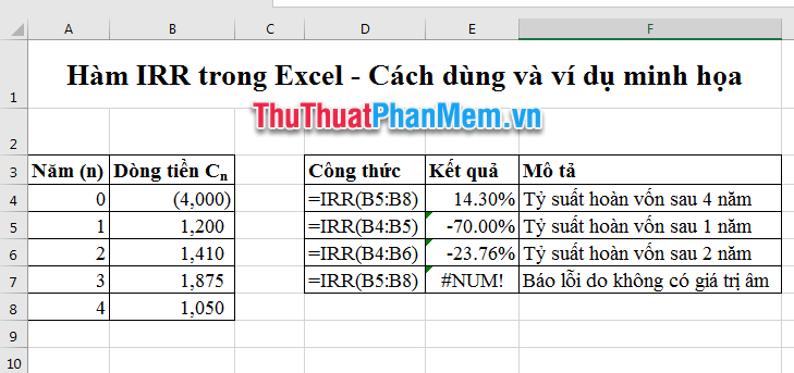
With the above example, if you use a manual calculation formula, it will take a lot of time to solve this problem. But if you use Excel, the result is just after 1s, you can even calculate the rate of return after 1 year, 2 years, 3 years .

You enter the above data sheet into the worksheet:

Excel will calculate the rate of return after any year you need.

In addition, you can enter the number in the IRR function, type any cell in the Excel worksheet = IRR ({- 4000,1200,1410,1875,1050}, 10%). The result is still 14.3%.

Good luck!