The quickest way to filter data by color in Google Sheets.

Although Google Sheets doesn't directly support color filtering, you can still filter data by color in two ways: using a code snippet or a Google Sheets add-on.

HOW TO FILTER DATA BY COLOR ON GOOGLE SHEETS

We will use the code to convert the cell color to hexadecimal code, then use Conditional Formatting to filter the color as desired.

Step 1: Open the Google Sheets spreadsheet you want to filter.

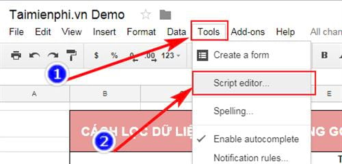
Step 2: Select Tools from the toolbar, then select Script Editor .

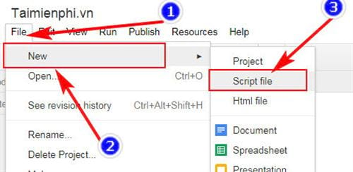
Step 3: Select File and then select New to create a new character encoding table.

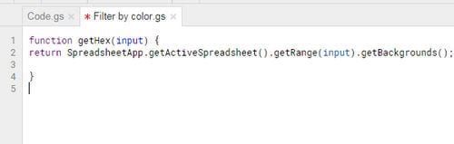
Step 4: Type in:

' function getHex(input) {

return SpreadsheetApp.getActiveSpreadsheet().getRange(input).getBackgrounds();

}'.

Step 5:  Return to the spreadsheet and enter the formula =getHex("B7:B11") into cell F7.

This formula will display the color codes of cells B7 through B11.

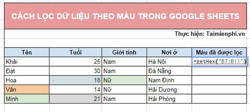
Step 6: After entering the formula, press Enter . The cell colors will be displayed as hexadecimal codes.

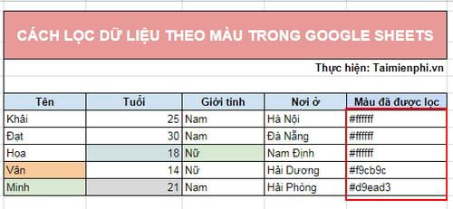
Step 7: Next, select Format > Conditional Formatting .

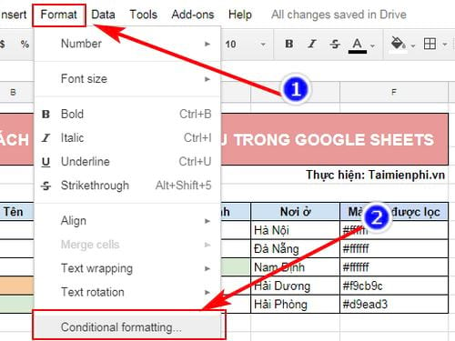
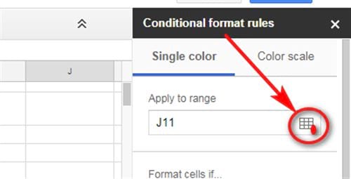
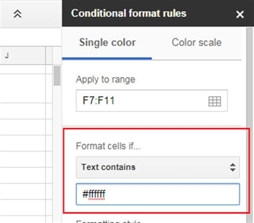
Step 8: In the "Apply to range" section , select the data range to filter from the filtered Color column by clicking the square box on the right.

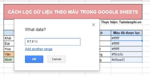
Next, select the data range you want to filter. Then press OK.

Step 9: Select Format cells if. > Text contains . Then, enter the color you want to filter, for example, #ffffff.

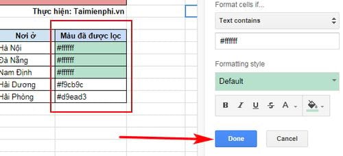
Step 10: Click Done to finish. The cells with the color #ffffff in the Filtered Colors column will be highlighted.

Above is a guide on how to filter data by color in Google Sheets. TipsMake hopes that this article will help you easily perform these steps to assist you in your work. If you are using Microsoft Excel and don't know how to filter duplicate data, you can refer to how to filter duplicate data in Excel here.