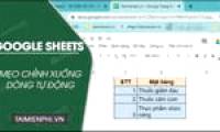
The quickest and simplest way to wrap text in Google Sheets.

Cells in Google Sheets can contain many characters, but when the number of characters in a cell exceeds the limit, the content will overflow into the adjacent cell if that cell is empty, or be hidden from view if the adjacent cell is not empty. In this case, line breaks are the most effective way to organize and display the full content in your cell in a scientific and logical manner. To understand this better, you can refer to the method of adding line breaks in Google Sheets shared by TipsMake below.

How to wrap text within a single cell in a Google Sheet on a computer or phone.

Note: To insert a line break or wrap text from any cell in Google Sheets, you need to follow one of the four methods below.

 

1. Wrap text in Google Sheets using a keyboard shortcut.

Step 1: Double-click the cell where you want to insert a line break so you can edit the content.

Step 2: Click the mouse at the location where you want to insert a new line.

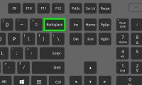
Step 3: Press and hold the key combination:

- Ctrl + Enter or Alt + Enter on Windows.
- Ctrl + Return or Alt + Return or ⌘ + Return on Mac.

Depending on the cell's content, you can create multiple line breaks within that cell using this method.

Step 4: Press Enter to complete.

Step 5: When you move to the next line, the height of all cells in the entire row will increase based on the changes in the cell. You can adjust the cells to best suit your needs.

Using Google Sheets, you'll often need to merge cells in a row or column and combine them into a single cell. This is especially useful when you want to create a header that spans multiple columns of a spreadsheet. The guide below will help you quickly merge cells in Google Sheets .

 

2. Wrap one cell on a single line in a Google Sheet using the Automatic Line Wrap tool.

Step 1: Click on the cell where you want to insert a line break and click the Automatic Line Break icon on the toolbar.

Step 2: Under the expanded menu that appears, you can choose from three options: Overflow , Line Break , and Trim . Click the Line Break icon in the middle to break the line.

The Overflow option will cause the content in your cell to overflow into other cells on the same line. Conversely, the Crop option will only display the content within the width of that cell; if the cell is too long, subsequent characters will be hidden.

Note: Google Sheets will adjust the cell height and display the text across multiple lines, effectively preventing the text from overflowing. However, this will not split your text into separate lines. If you look at the formula bar, the text will still be displayed on a single line.

 

3. Create a new line in Google Sheet using the Copy-Paste command.

Step 1: To create a line break using the Copy-Paste command, you need to use text editing software such as Notepad or any other text editor. Enter the content you want to place inside the cell and create a line break by pressing Enter as usual.

Step 2: Double-click the cell in Google Sheet and paste the content you just copied from Notepad into that cell.

Note: Google Sheets will automatically wrap text pasted into cells because the wrapping has already been done in the text editing software. Unless you double-click a specific cell to paste the text, it will be entered into separate cells as illustrated.

 

4. Use the CHAR function to add line breaks and shorten lines in Google Sheets.

If you're looking for a way to use formulas to add line breaks in Google Sheets, the CHAR function is a simple formula to do this.

Step 1: Click on the cell containing the content you want to wrap to the next line and press the = key to start entering the formula:

"First line content" & CHAR(10) & "newline content"

Step 2: Press Enter and your content will appear in two lines.

Step 3: If you want to break lines multiple times, simply divide your content with the character string & CHAR(10) & between the lines you need to break on the formula bar.

By default, data in a Google Sheet file can be changed and edited by everyone with access rights. However, if you don't want anyone to arbitrarily change, edit, or delete existing content in the file, you can set permissions for each person in the Google Sheet file. If you don't know how, the article on how to set editing permissions for spreadsheets in Google Sheets will provide you with a lot of information.

In summary, TipsMake has introduced to readers how to wrap text in Google Sheets with detailed steps. Hopefully, with this trick, you can easily handle long content and paragraphs in Google Sheet cells. If you have any questions, please leave a comment below for clarification.