MIRR Function in Excel: Syntax and Examples

This article provides a clear overview of MIRR Function in Excel, with the main facts, useful context, and practical details organized for easy reading.

Instructions for Using the MIRR Function

What This Feature Does

Perform the calculation of the internal rate of return adjusted for periodic cash flow. Not only that, but MIRR allows calculating the cost and interest if reinvested.

Syntax

MIRR (values, finance_rate, reinvest_rate) .

Arguments

- values: Include payments, including negative values. This includes initial expenses, loans, etc.

- finance_rate: Interest paid on loans in the cash flow.

- reinvest_rate: Interest received when reinvesting.

Example

Give the following data table:

Calculate:

- Calculate the interest rate of the investment after a period of 3 years.

- Calculate the interest rate of the investment after a period of 5 years.

- Calculate the interest rate of the investment after a period of 5 years and use the reinvestment with the interest rate of 12%.

Perform the problem:

1. Interest Rate of the Investment After 3 Years

in the target cell enter the formula: = MIRR (D5: D8, D11, D12) .

Result:

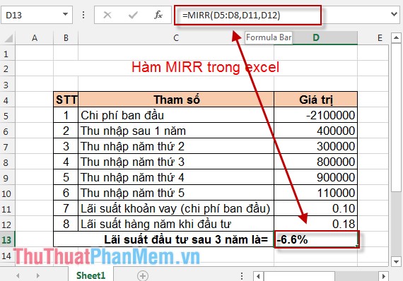
So after 3 years, the interest rate = -6.6% ? The investment after 3 years has no interest.

2. Interest Rate After 5 Years

in the target cell enter the formula: = MIRR (D5: D10, D11, D12) .

Results after calculation:

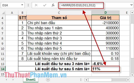
So the investment after 5 years is profitable and the interest rate is 11% of the capital.

3. Interest Rate Received After 5 Years with Reinvestment Receives Interest Rate of 12%

in the target cell enter the formula: = MIRR (D5: D10, D11.12%) .

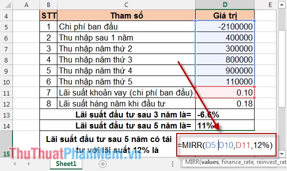
Result:

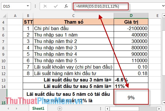
The interest rate after 5 years of reinvestment with the interest rate of 12% = 9% <11% ? The effective reinvestment is not high, you should consider.