How to Integrate Large Data Sets in Excel

Part 1 of 3:

Preparing

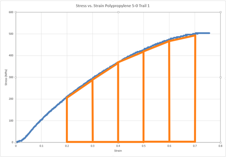Understand the basics of the trapezoid rule. This is how the integral will be approximated. Imagine the stress-strain curve above, but separated into hundreds of trapezoidal sections. Each section's area will be added to find the area under the curve.
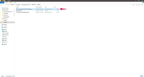Load the data into Excel. You can do this by double-clicking on the .xls or .xlsx file that is exported by the machine.
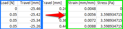Convert the measurements into a usable form, if needed. For this particular data set, it means converting the tensile machine measurements from "Travel" to "Strain", and "Load" to "Stress", respectively. This step may require different calculations or may not be needed at all, depending on the data from your machine.

Part 2 of 3:

Setting Up Your Dimensions

Determine which columns will represent the width and height of the trapezoid. Once again, this will be determined by the nature of your data. For this set, "Strain" corresponds to the width and "Stress" corresponds to the height.
Click on a blank column and label it "Width". This new column will be used to store the width of each trapezoid.
Select the empty cell below "Width" and type "=ABS(". Type it exactly as shown, and do not stop typing in the cell yet. Note that the "typing" cursor is still flashing.
Click on the second measurement corresponding to the width, then press the - key.
Click on the first measurement in the same column, and type in the closing parenthesis, and press ↵ Enter. The cell should now have a number in it.
Select the newly created cell and move the mouse cursor to the bottom right corner of the cell directly below, until a cross appears.
1. Once it appears, left click, hold, and drag the cursor down.
2. Stop at the cell directly above the last measurement. Numbers should populate all the selected cells after.
Click on a blank column and label it "Height" directly next to the "Width" column.
Select the column underneath the "Height" label, and type "=0.5*(". Once again, do not exit the cell just yet.
Click the first measurement in the column corresponding to the height, then press the + key.
Click on the second measurement in the same column, and type the closing parenthesis, and press ↵ Enter. The cell should have a number in it.
Click on the newly created cell. Repeat the same procedure you did before to apply the formula to all the cells in the same column.
1. Once again, stop at the cell before the last measurement. Numbers should appear in all the selected cells.

Part 3 of 3:

Calculating the Area

Click on a blank column and label it "Area" next to the "Height" column. This will store the area for each trapezoid.
Click on the cell directly underneath "Area", and type "=". Once again, do not exit the cell.
Click on the first cell in the "Width" column, and type an asterisk (*) directly after.
Click on the first cell in the "Height" column, and press ↵ Enter. A number should now appear in the cell.
Click on the newly created cell. Repeat the procedure you applied before again to apply the formula to all the cells in the same column.
1. Once again, stop at the cell before the last measurement. Numbers should appear in the selected cells after this step.
Click on a blank column and label it "Integral" next to the "Area" column.
Click on the cell below "Integral", and type in "=SUM(", and do not exit the cell.
Click on the first cell under "Area", hold, and drag downwards until all the cells in the "Area" column are selected, then press ↵ Enter. A number under "Integral" should appear, and will be the answer.

David Pac

Update 05 March 2020

You should read it

May be interested

How to Compare Data in Excel
this wikihow teaches how to compare different sets of data in excel, from two columns in the same spreadsheet to two different excel files. highlight the first cell of a blank column. when comparing two columns in a worksheet, you'll be...
CORREL function - The function returns the correlation coefficient between two data sets in Excel
correl function: the function returns the correlation coefficient between two data sets. correlation coefficient is used to determine the relationship between two attributes. syntax: correl (array1, array2)
Find and delete duplicate data in Excel
find and delete duplicate data in excel. in the process of working with excel spreadsheets, there will be excel files with large amounts of data so duplication of data is very common. there are cases where duplicate data is useful, but sometimes values are
How to find the Nth value in Excel
when working with data analysis tables in excel, there will often be a request to find the largest value, the second largest value, or the smallest value, ...
How to use the FILTER function in Excel
if you regularly work with data sets in excel, you know how important it is to be able to quickly find the information you need.
Filter duplicate data, delete duplicate data in Excel
for excel files with large log volumes, duplication of data is very common. so i introduce to you how to filter duplicated data with tools available in excel.
COVARIANCE.S function - Returns the covariance pattern, the average of product deviations for each pair of data points in two data sets in Excel
covariance.s function: returns the covariance, the product of the deviations for each pair of data points in two data sets syntax: covariance.s (array1, array2)
Filter data that doesn't overlap in Excel - Filter for unique values in Excel
in a spreadsheet with large information data, it is difficult to check and filter which data is duplicated and which is not. especially if you manually / eye check it is very time consuming. thankfully, excel has a tool that makes it possible for users to filter for duplicate values in excel (unique values).
Add captions to spreadsheets in Excel 2013
when setting up a spreadsheet with hundreds, thousands of data boxes, these data boxes will be linked together but with a large number of such cells even you may forget some information about the box yourself. which data is in this record, what documents ... if you share this spreadsheet with others, the problem is even more complicated.
How to Group and Outline Excel Data
this wikihow teaches you how to group a section of data in excel so that you can hide it from the document. this is helpful if you have a large document with lots of data. you can group and outline data in excel on both windows and mac...

How to Integrate Large Data Sets in Excel

Preparing

Setting Up Your Dimensions

Calculating the Area

You should read it

May be interested

Office information