How to Create a Line of Spheres Pattern in Microsoft Excel

The Tutorial

1. How to Create a Line of Spheres Pattern in Microsoft Excel Picture 1
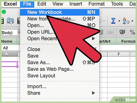
   Start a new workbook by saving the previous workbook from How to Create the One Sphere Pattern in Microsoft Excel under a new name. Save the workbook into a logical file folder.
2. How to Create a Line of Spheres Pattern in Microsoft Excel Picture 2
   Add the first of two tables. The first one creates the line the chart will follow.

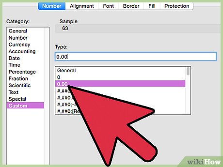
   1. Enter 63 to cell AD1 and Format Cell Number Number Custom "Degrees "0.00 and Insert Name Define name Degrees to cell $AD$1. 90 degrees is a problem, as is 0 and 180 and 360, but otherwise, it works well..
   2. Enter Slope into cell AE1 and into cell AE2 Insert Name Define Name Slope to cell $AE$2 and enter the formula w/o quotes "=TAN(Degrees*PI()/180)"
   3. Enter Factor_Up into cell AF1 and enter w/o spaces 2.102 594 6851 1947 into cell AF2 and enter =2.43189347013788*S_COUNT/24 into cell AF3.
   4. Enter b_ into cell AG1 and enter w/o spaces -0.939 692 620 785 908 into cell AG2. Enter b_YN into cell AG3 and N into cell AG4 and Insert Name Define b_YM to cell $AG$4 and b_ to cell $AG$2. Enter 0 into cell AG2.
   5. Enter New x  into cell AE6 and New y into cell AF6.
   6. Enter 0 into cell AE7 and Format Fill yellow and do Font red bold and centered horizontal. Enter "=1+COS(Degrees*PI()/180)" into cell AE1447 and Format Fill yellow and do Font red bold and centered horizontal.Edit Go To cell range AE8:AE1446 and with AE8 active enter the formula w/o quotes "=($AE$1447-$AE$7)/1439+AE7" and Edit Fill Down.
   7. Edit Go To cell range AF7:AF1447 and enter w/o quotes with AF7 active the formula "=Factor_Up*(Slope*AE7)+IF(b_YN="N",0,b_)". Factor_Up will stretch or shrink the line in theory for its y values. The b-intercept may be set to 0 in b_ or negated via N in b_YN while retaining a previous value in b_, or both.
   8. Select AG1448 and enter Min, AG1449 and enter Max, AG1450 and enter Goal, AG1451 and enter Bu changing Factor_Up, and select AG1452 and enter Goal by changing b_.
   9. Select AE1448 and enter "=MIN(AE7:AE1447)" and select AE1449 and enter "=MAX(AE7:AE1447)". Copy AE1448:AE1449 and Paste to AF1448. Select AF1450 and enter 6, then enter into cell AF1451 "=AF1450-AF1447" which is the set to zero cell, when we want to change AF7 (it has to be a value first) to equal 0 by changing Factor_Up.
   10. Select cell AE1452 and enter "=1-AE7" which is what we want to equal zero when we want cell AE7 to equal 1 (therefore the line would start at {1,0} instead of at {0,0}) -- it's there for user discretion and is utilized by changing AE7 simply to 1 now -- it used to also depend on Factor_Up or b_. Select cell AF1452 and enter "=0-AF7" which is the Goal when we want to change AF7 to 0 by changing b_.
   11. Select cell AD1454 and enter Chart has, then select cell AE1454 and input 1440, then select AF1454 and enter rows. Select AD1455 and enter Divided by, and select AE1455 and enter 24 and select AF1455 and enter Spheroids. Enter Equals into cell AD1456 and "=AE1454/AE1455" into cell AE1456, with the answer being 60.
   12. Enter 3 in cell AE1457 and into cell AD1457 enter Number of Spheroids to Chart and Format Cells Font bold size 14 and alignment right. Aligned left, select cell AB1458 and enter the formula with quotes ="So if "&AE1457&" Spheroids are wanted, then adjust the series in the chart formula bar to the first "&AE1456*AE1457&" rows."
   13.  and Format cells Font bold size 12. By calculation, the user may select which three spheroids to chart, adjusting for the fact that the series starts in row 7. So, if for example, the last 3 spheroids were wanted, the user would subtract 180 from 1447 and chart only that row (1267) up to row 1447. The user would then adjust the axes according to the demands of the rest of their graphic layout. Changing the number of spheroids in S_Count works, but only over a limited range of values -- this solution always works.
3. How to Create a Line of Spheres Pattern in Microsoft Excel Picture 3
   The second table is one seen before -- it's the LOOKER table. In the time it'd take to find which articles it's in and hope the reader has done one, it can be done already.

   1. Edit Go To AI7:AI70 and enter 1 into AI7 and Edit Fill Series Column Linear Step Value 1.
   2. Edit Go To AJ7:AJ70 and enter .125 and Edit Fill Down.
   3. Edit Go To AK7:AK70 and enter "=AI8*$AK$36/$AI$36" and Edit Fill Down. Select cell AK36 and input .125 and select AK70 and enter 0.
   4. Edit Go To cell range AI7:AK79 and Insert Name Define Name Looker to cell range $AI$7:$AK$70. Select cell AK6 and enter the header LOOKER.
4. How to Create a Line of Spheres Pattern in Microsoft Excel Picture 4
   Complete all changes in the upper Defined Variables section.

   1. Enter On=0,Off=1 cell A4 = 1
   2. Enter Spirallic_YN N into cell A6.
   3. Enter Adjuster = 1 in cell B1.
   4. Enter TURNS =S_COUNT/24*60 in cell B2.
   5. Enter AdjRows = 1440 in cell B3.
   6. Enter t = -308,160 in cell B4.
   7. Enter S's Count = 24 in cell C1.
   8. Enter Designer =VLOOKUP(S_COUNT,SPHEROIDS_COUNT_LOOKER,2) in cell C2.
   9. Enter Var = 12 in cell C3.
   10. Enter Cc =-0.25*PI()/C3 in cell C4.
   11. Enter db = 4.5 in cell C5.
   12. Enter top =ROUND((-B4*PI())+(Adj),0) into cell D1.
   13. Enter Divisor = 40,571,226,658.4877 in cell D2.
   14. Enter AAA = 0 in cell D3.
   15. REVERSION: Enter Factor =IF(ISNA(VLOOKUP(S_COUNT,LOOKER,2)),0.125,VLOOKUP(S_COUNT,LOOKER,3))
   16. REVERSION: Enter Base 1712 into cell D5 and Format Cell Number Number "Base "0
   17. Enter Power = 1 in cell E1.
   18. NEW: Enter 60 into cell E2 (FFF)
   19. Enter YN = N for Part-Cycle in E3.
   20. Enter YN = N for Molecules in cell E4.
   21. G1 GMSL = 0.381966011250105
   22. G2 GMLL = 0.618033988749895
   23. H1 = .98 and J1 = .96. H2 Sync1 =H1/GML and J2 Sync2 =J1/GMSL.
5. How to Create a Line of Spheres Pattern in Microsoft Excel Picture 5
   Complete all changes in the mid-range Columnar Formulas section.

   1. The long formula in cells A7:A1447 has apparently not changed.
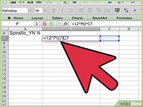
   2. REVERSION: The formula in cell B7 is =12*PI()*C7
   3. Check that the formulas in cell range B8:B1447 are still =((B7+(-TOP*2)/(AdjRows)))*$B$1
   4. Check that the formula in C7 is =ROUND(-EXP((PI()^2)+(Cc*-(db))),0)+Designer
   5. Check that the formulas in cell range C8:C1447 are still =C7 (i.e. relatively equivalent).
   6. REVERSION: Enter the formulas in D7:D1447 =COS((ROW()-7)*PI()/180*Factor) and Edit Fill Down.
   7. REVERSION: Edit the formulas in E7:E1447 =SIN((ROW()-7)*PI()/180*Factor) and Edit Fill Down.
   8. NEW: Enter the formula into cell range F7:F1447=IF(A7=0,F6,(((SIN(B7/(C7*2))*GMLL*COS(B7)*GMLL*(COS(B7/(C7*2)))*GMLL)+AE7)))*IF(Spirallic_YN="Y",SPIRALLIC,1)  and Edit Fill Down.
   9. NEW: Enter the formula into cell range G7:G1447 =IF(A7=0,G6,(((SIN(B7/(C7*2))*GMLL*SIN(B7)*GMLL*(COS(B7/(C7*2)))*GMLL)+AF7))*IF(Spirallic_YN="Y",SPIRALLIC,1)) and Edit Fill Down.
   10. Check the formula in H7 is =F7*GMLL*Sync1
   11. Check the formula in I7 is =G7*GMLL*Sync1
   12. Check the formula in J7 is =F7*GMSL*Sync2
   13. Check the formula in K7 is =G7*GMSL*Sync2
   14. The lookup tables have not changed, except for the following, perhaps:
   15. Check the value in cell U4, ADJ_Y is 0.141592653589793
   16. The value in FFF, cell AA7, should read 60.
   17. NEW? Under Radius in column Z  are variable amounts. The formula in cell Z7 is =ROUND(((X7-V7)^2+(Y7-W7)^2)^0.5,4) and this is relatively the same in Z8 and Z1447.
   18. Check for errors. If there are any, there are none in the example workbook. Please see the Warnings section below for help, if or as needed.

Explanatory Charts, Diagrams, Photos

1. (dependent upon the tutorial data above)

1. How to Create a Line of Spheres Pattern in Microsoft Excel Picture 6
   Create the Chart.

   1. Edit Go To cell range F7:G1447 and, using either the Chart Wizard or the Ribbon, select Charts, All/Other, Scatter-Smoothed Line Scatter. A chart will appear atop the data unless using Chart Wizard, in which case a new Chart sheet will appear.
   2. Assuming the former case, Copy or Cut the chart from atop the data and paste it to the Chart worksheet, then expand it by hovering over the lower right corner until the cursor becomes a double-headed arrow and clicking to drag the Chart Area until about a 6" wide by 4" tall rectangle is formed.
   3. Using Chart Layout, select the Horizontal Axis and set Minimum to -1.5  Maximum to 3.0, Major unit to 1.5. Minor unit to .3 and Vertical Axis crosses at 0.0, in Base 10, OK.
   4. Using Chart Layout, select the Vertical Axis and set Minimum to -1, Maximum to 7, Major unit to 1.0. Minor unit to .3 and Vertical Axis crosses at 0.0, in Base 10, OK. It's done according to Min Max row formulas at the bottom of columns F and G or AE and AF kept there for just such an occasion.
   5. The axes may now be safely eliminated as well as any grid lines and legend.
2. How to Create a Line of Spheres Pattern in Microsoft Excel Picture 7
   How to Create a Line of Spheres Pattern in Microsoft Excel Picture 8
   Finished! Your chart should resemble the one above. #

   1. How to Create a Line of Spheres Pattern in Microsoft Excel Picture 9

Helpful Guidance

1. Make use of helper articles when proceeding through this tutorial:

   1. See the article How to Create a Spirallic Spin Particle Path or Necklace Form or Spherical Border for a list of articles related to Excel, Geometric and/or Trigonometric Art, Charting/Diagramming and Algebraic Formulation.
   2. For more art charts and graphs, you might also want to click on Category:Microsoft Excel Imagery, Category:Mathematics, Category:Spreadsheets or Category:Graphics to view many Excel worksheets and charts where Trigonometry, Geometry and Calculus have been turned into Art, or simply click on the category as appears in the upper right white portion of this page, or at the bottom left of the page.